Mesh geometry

The vcg_* and mris_* families are ravetools’ low-level geometry layer. They are the building blocks that the surface pipelines are assembled from, and they are usable directly. This article walks the whole family, grouped the way the README table groups it: construct, measure, repair, smooth, query, subset, and draw.

Every mesh these functions return carries the ravetools_mesh3d class, which is an rgl-style mesh3d – a 3 x n vertex matrix vb and a 3 x m one-based triangle matrix it – so plot() renders it in base R graphics with no rgl dependency. ensure_mesh3d coerces the other common surface formats (fs.surface from freesurferformats, ieegio_surface from ieegio, surf.asc) into the same layout, so a FreeSurfer surface drops into any function below.

1. Two primitives

The cheapest way to get a mesh is to make one. vcg_sphere returns a subdivided icosphere of unit radius centered at the origin, and plane_geometry returns a flat triangulated grid in the z = 0 plane.

sphere <- vcg_sphere(sub_division = 4)
sphere
#>  mesh3d object with 2562 vertices, 5120 triangles.

plane <- plane_geometry(width = 2.6, height = 2.6, shape = c(40, 40))
plane
#>  mesh3d object with 1600 vertices, 3042 triangles.

shape counts vertices per side, so a 40 x 40 grid is 39 x 39 cells and twice that many triangles. Tilt the plane and lift it, and it slices through the sphere:

tilt <- new_matrix4()$make_rotation_y(25 * pi / 180)$to_array()
plane$vb <- (tilt %*% rbind(plane$vb[1:3, ], 1))[1:3, ] + c(0, 0, 0.35)

new_matrix4 is one of the in-place geometry classes (new_vector3, new_matrix4, new_quaternion); to_array hands back the plain 4x4 matrix.

Faces alone do not carry orientation. vcg_update_normals computes per-vertex normals, which the smoothing, projection, and ray-casting routines all read:

plane <- vcg_update_normals(plane, weight = "area")
dim(plane$normals)
#> [1]    4 1600

2. Asking questions about geometry

Three functions answer “where is this thing relative to that thing”, and they trade accuracy against cost differently.

Exact collision

vcg_detect_collision reports, for every element of y, whether it comes within radius of x, together with the exact minimum distance. Either side can be a point cloud, a chain of connected line segments, or a triangular mesh, so one call covers all nine pairings. Both sides here are meshes, so answers come back one per triangle of y:

cut <- vcg_detect_collision(sphere, plane, radius = 0.02)
cut$summary$y$unit_type
#> [1] "face"
sum(cut$hit_unit)
#> [1] 307
head(cut$representation)
#>   unit index    distance x_index
#> 1  354     2 0.019227119     141
#> 2  355     2 0.019227119     141
#> 3  356     2 0.017633209     144
#> 4  357     2 0.018250201     131
#> 5  358     1 0.018250201     131
#> 6  424     2 0.005326802     349

representation has one row per hit: unit is the plane triangle, index is the vertex of that triangle nearest the sphere, distance is the true minimum distance, and x_index is the sphere face that was hit. Keeping those triangles gives the intersection band as a mesh in its own right:

band <- plane
band$it <- plane$it[, which(cut$hit_unit), drop = FALSE]
band
#>  mesh3d object with 1600 vertices, 307 triangles.

The radius argument makes this a proximity test rather than a contact test. Raising it thickens the band, because more triangles fall inside the tolerance:

vapply(c(0.02, 0.1, 0.3), function(r) {
  sum(vcg_detect_collision(sphere, plane, radius = r)$hit_unit)
}, 0L)
#> [1]  307  760 1850

Line segments are the case worth knowing about, because that is how diffusion streamlines and electrode shafts arrive. Several chains share one matrix and are delimited by rows of NA:

streamlines <- rbind(
  cbind(seq(-3, 3, by = 0.5), 0, 0),
  c(NA, NA, NA),
  cbind(seq(-3, 3, by = 0.5), 5, 0)
)
res <- vcg_detect_collision(sphere, streamlines,
                            mode_y = "segments", radius = 0.1)
res$hit_unit
#> [1]  TRUE FALSE
res$representation
#>   unit index distance x_index
#> 1    1     4        0    1894

The first chain runs through the sphere and the second passes well clear of it. test_level controls how hard the scan works: "element" (the default) measures every segment and reports the closest, "unit" stops at the first hit inside each chain, and "whole" stops at the first hit anywhere and answers only the yes-or-no question:

vcg_detect_collision(sphere, streamlines, mode_y = "segments",
                     radius = 0.1, test_level = "whole")$collide
#> [1] TRUE

Finally, include_interior decides whether geometry buried inside a closed x counts as a collision even when it never approaches the surface. The center of the sphere is one unit away from every point of it:

center <- rbind(c(0, 0, 0))
vcg_detect_collision(sphere, center, radius = 0.1)$collide
#> [1] FALSE
vcg_detect_collision(sphere, center, radius = 0.1,
                     include_interior = TRUE)$collide
#> [1] TRUE

That test uses ray casting, so it needs x to be watertight with coherently oriented faces – see vcg_fix_defects below for repairing one that is not.

Nearest neighbors

vcg_kdtree_nearest builds a K-D tree over target and, for each point of query, returns the k closest target points and their distances. Unlike vcg_detect_collision it measures to the nearest vertex, not to the surface, so it is an approximation – a cheaper one that is usually good enough, and the right tool when the identity of the nearest vertex is what is wanted:

kd <- vcg_kdtree_nearest(target = sphere, query = plane, k = 1)
str(kd)
#> List of 2
#>  $ index   : int [1:1600, 1] 1843 1843 1843 1845 1845 1847 1847 1887 1887 1887 ...
#>  $ distance: num [1:1600, 1] 0.972 0.923 0.877 0.832 0.786 ...
range(kd$distance)
#> [1] 0.007727357 0.972278178

Asking for more than one neighbor widens both matrices to k columns, which is how you get a local neighborhood to average over:

kd3 <- vcg_kdtree_nearest(target = sphere, query = plane, k = 3)
head(kd3$index)
#>      [,1] [,2] [,3]
#> [1,] 1843 1835 1833
#> [2,] 1843 1833 1835
#> [3,] 1843 1844 1845
#> [4,] 1845 1844 1843
#> [5,] 1845 1844 1847
#> [6,] 1847 1845 1844

Both arguments accept either a mesh or a plain n x 3 matrix, and 2D points work as well as 3D.

Ray casting

vcg_raycaster shoots a ray from each origin along each direction and reports the first face it meets. Lift the plane clear of the sphere and drop a ray straight down from every vertex:

above <- plane$vb
above[3, ] <- above[3, ] + 1.8
rays <- vcg_raycaster(sphere, ray_origin = above, ray_direction = c(0, 0, -1))
str(rays[c("has_intersection", "distance", "face_index")])
#> List of 3
#>  $ has_intersection: logi [1:1600] FALSE FALSE FALSE FALSE FALSE FALSE ...
#>  $ distance        : num [1:1600] NA NA NA NA NA NA NA NA NA NA ...
#>  $ face_index      : int [1:1600] NA NA NA NA NA NA NA NA NA NA ...
sum(rays$has_intersection)
#> [1] 780

Rays whose origin lies over the sphere’s silhouette hit it; the rest report has_intersection = FALSE, NA for distance and face_index, and an intersection column that should be ignored. both_sides = TRUE also searches backwards along the ray, and max_distance caps how far it travels.

The hits form a point cloud, which is a mesh with vertices and no faces:

pierce <- structure(
  list(vb = rays$intersection[, rays$has_intersection, drop = FALSE]),
  class = "mesh3d"
)

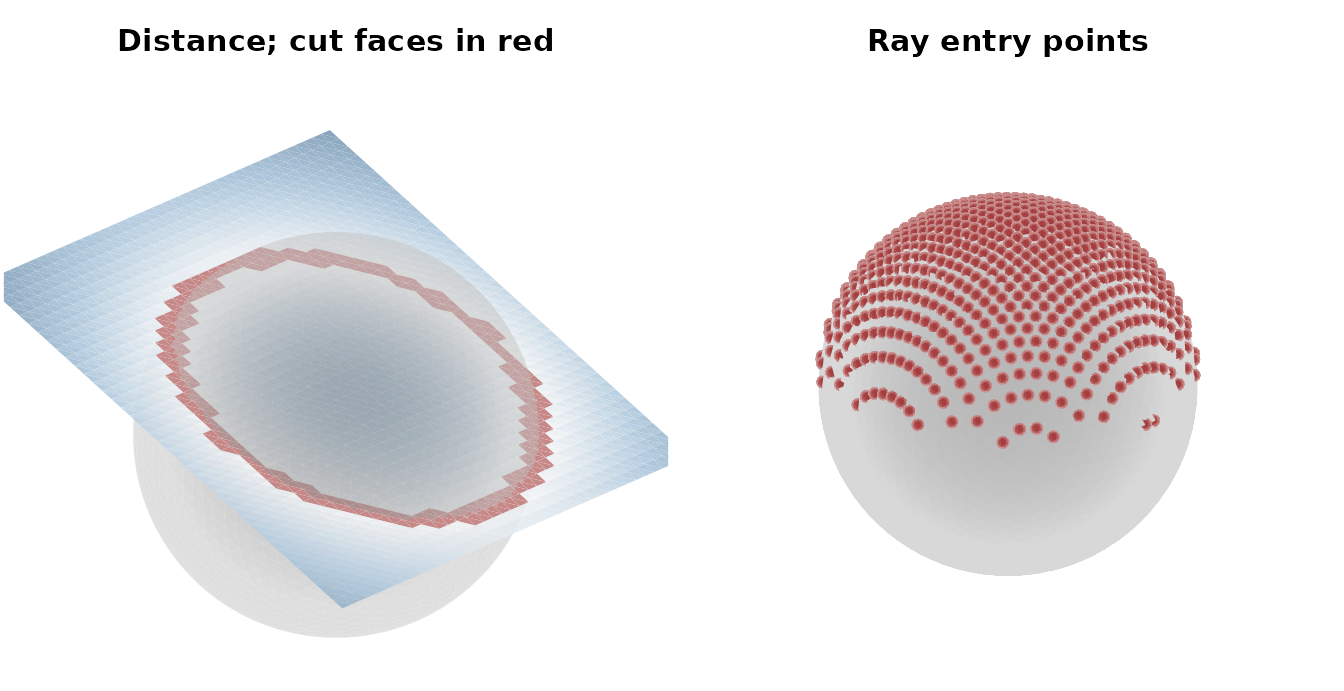
Putting the three answers side by side:

col <- color_ramp_continuous(kd$distance[, 1],
                             cmap = c("#f2f2f2", "#7fa8c9", "#2c5f8a"))

graphics::par(mfrow = c(1, 2), mar = c(0.1, 0.1, 2.1, 0.1), cex.main = 0.95)
plot_mesh_polygon(
  list(sphere, plane, band),
  col = list("gray55", col, "#a33a3a"), alpha = c(0.5, 0.92, 1),
  eye = c(3.5, -4, 2.2), up = c(0, 0, 1), zoom = 1.15,
  shadow_color = "white", ambient_intensity = 0.55,
  main = "Distance; cut faces in red"
)
plot_mesh_polygon(
  list(sphere, pierce),
  col = list("gray72", "#a33a3a"), cex = 0.03,
  eye = c(3.5, -4, 2.2), up = c(0, 0, 1), zoom = 0.68,
  shadow_color = "white", ambient_intensity = 0.55,
  main = "Ray entry points"
)

3. Building a mesh from a volume

Real surfaces come from volumes. vcg_isosurface runs marching cubes over a 3D array and returns the triangulation, mapping voxel indices into RAS through vox_to_ras:

data("left_hippocampus_mask", package = "ravetools")
dim(left_hippocampus_mask)
#> [1] 51 48 38

raw_mesh <- vcg_isosurface(left_hippocampus_mask)
raw_mesh
#>  mesh3d object with 4318 vertices, 8652 triangles.

mesh_from_volume wraps the same step together with re-sampling and smoothing, which is convenient when the goal is a display surface rather than an exact level set:

smoothed <- mesh_from_volume(
  left_hippocampus_mask, output_format = "rgl", threshold = 0.5,
  remesh = TRUE, remesh_voxel_size = 1, smooth = TRUE, verbose = FALSE
)
smoothed
#>  mesh3d object with 4148 vertices, 8292 triangles.

mris_make_surfaces is the fourth constructor. It deforms an existing surface along the intensity gradient of a volume to produce paired white and pial surfaces, the way a cortical reconstruction does.

4. Measuring and diagnosing

Before doing anything to a mesh it is worth asking what shape it is in. vcg_count_edge_defects counts the two things that break most algorithms:

vcg_count_edge_defects(raw_mesh)
#> $boundary_edges
#> [1] 40
#> 
#> $nonmanifold_edges
#> [1] 0
#> 
#> $is_closed_manifold
#> [1] FALSE

Forty boundary edges means the marching-cubes output has holes, so it is not closed. vcg_mesh_volume says so itself rather than quietly returning a number that means nothing:

vcg_mesh_volume(raw_mesh)
#> Warning in vcgVolume(meshintegrity(mesh)): Mesh is not watertight! USE RESULT
#> WITH CARE!
#> [1] 5517.25
vcg_average_edge_length(raw_mesh)
#> [1] 0.9971679
vcg_max_edge_length(raw_mesh)
#> [1] 1.414214

The two edge-length measures are the ones to check before any operation with a length parameter, since they say what scale the mesh is sampled at.

mris_curvature returns the four standard curvature fields per vertex – mean, Gaussian, and the two principal curvatures:

curv <- mris_curvature(raw_mesh)
str(curv)
#> List of 4
#>  $ mean    : num [1:4318] -0.468 -0.69 -0.509 -0.284 -0.334 ...
#>  $ gaussian: num [1:4318] 0.138 0.43 0.1937 0.061 0.0479 ...
#>  $ k1      : num [1:4318] -0.183 -0.475 -0.2536 -0.1433 -0.0816 ...
#>  $ k2      : num [1:4318] -0.754 -0.905 -0.764 -0.426 -0.587 ...

5. Repairing and re-meshing

vcg_fix_defects merges duplicate vertices, fills holes, and reorients faces, and it reports what it did in an info attribute:

mesh <- vcg_fix_defects(raw_mesh, verbose = FALSE)
info <- attr(mesh, "info")
info[c("boundary_edges_before", "boundary_edges_after",
       "holes_filled", "is_closed_manifold")]
#> $boundary_edges_before
#> [1] 40
#> 
#> $boundary_edges_after
#> [1] 0
#> 
#> $holes_filled
#> [1] 10
#> 
#> $is_closed_manifold
#> [1] TRUE

# the same call that warned above, now on a closed surface
vcg_mesh_volume(mesh)
#> [1] 5517.25

The mesh is a closed manifold now, so its volume is trustworthy and include_interior collision tests will work on it. Center it for the plots that follow:

mesh$vb[1:3, ] <- mesh$vb[1:3, ] - rowMeans(mesh$vb[1:3, ])

Four routines change the sampling. They differ in what they preserve:

uniform  <- vcg_uniform_remesh(mesh, voxel_size = 1, verbose = FALSE)
split    <- vcg_subdivision(mesh, method = "edge")
capped   <- vcg_subdivide_max_edge_length(mesh, max_edge_len = 0.8)
isotropic <- mris_remesh(mesh, target_edge_length = 1.5, verbose = FALSE)

data.frame(
  method = c("input", "vcg_uniform_remesh", "vcg_subdivision",
             "vcg_subdivide_max_edge_length", "mris_remesh"),
  vertices = c(ncol(mesh$vb), ncol(uniform$vb), ncol(split$vb),
               ncol(capped$vb), ncol(isotropic$vb)),
  avg_edge = round(vapply(list(mesh, uniform, split, capped, isotropic),
                          vcg_average_edge_length, 0), 3),
  max_edge = round(vapply(list(mesh, uniform, split, capped, isotropic),
                          vcg_max_edge_length, 0), 3)
)
#>                          method vertices avg_edge max_edge
#> 1                         input     4318    0.997    1.414
#> 2            vcg_uniform_remesh     4161    0.988    1.717
#> 3               vcg_subdivision    17326    0.498    0.707
#> 4 vcg_subdivide_max_edge_length    12784    0.566    0.791
#> 5                   mris_remesh     1121    1.663    3.127

vcg_uniform_remesh re-samples through a distance field on a voxel grid, so it also repairs topology at the cost of exact geometry. vcg_subdivision splits every edge, doubling resolution everywhere. vcg_subdivide_max_edge_length splits only edges above a threshold, leaving well-sampled regions alone. mris_remesh implements the isotropic re-meshing of Botsch and Kobbelt (2003), driving every edge toward one target length, and is the one to reach for when downstream code cares about triangle quality.

6. Smoothing and deforming

Two smoothers come from vcglib and one from the cortical-surface literature:

taubin <- vcg_smooth_explicit(mesh, type = "taubin", iteration = 10)
implicit <- vcg_smooth_implicit(mesh, lambda = 0.2, degree = 2)
fs_style <- mris_smooth(mesh, niterations = 20L)

vapply(list(mesh, taubin, implicit, fs_style), vcg_mesh_volume, 0)
#> [1] 5517.250 5526.756 5419.094 4496.284

vcg_smooth_explicit applies a per-vertex Laplacian step repeatedly; type = "taubin" alternates a positive and a negative step so the surface does not shrink. vcg_smooth_implicit solves for the smoothed positions in one sparse solve, which is stable at much larger lambda. Both preserve the vertex count; only the positions move.

mris_inflate goes further, flattening the folds while preserving total surface area. It also returns the sulc depth field – how far each vertex traveled – which is what makes an inflated surface readable:

inflated <- mris_inflate(fs_style, n_averages = 4L, niterations = 8L,
                         scale_brain = FALSE, verbose = FALSE)
names(inflated)
#> [1] "mesh" "sulc"
range(inflated$sulc)
#> [1] -4.911788  4.436476

mris_sphere continues the deformation all the way onto a sphere of target_radius, which is the mapping that surface-based registration is built on. How close it gets is worth checking, because the residual spread in vertex radius is the honest measure of convergence:

spherical <- mris_sphere(fs_style, target_radius = 100, verbose = FALSE)
radius <- sqrt(colSums(spherical$vb[1:3, ]^2))
c(min = min(radius), max = max(radius), cv = stats::sd(radius) / mean(radius))
#>          min          max           cv 
#>  90.34295945 112.17180004   0.01515924

Under two percent here. Both mris_inflate and mris_sphere were designed for cortical surfaces, where the input is large, smooth, and genuinely sphere-like; a small closed structure such as this hippocampus maps only approximately, and raising niterations past the default makes it worse rather than better on such an input.

Mapped side by side with mean curvature, the first two stages show what inflation preserves:

curv <- mris_curvature(fs_style)
lim <- stats::quantile(abs(curv$mean), 0.95)
curv_col <- color_ramp_continuous(
  curv$mean, clim = c(-lim, lim),
  cmap = c("#2c5f8a", "#f2f2f2", "#a33a3a")
)

graphics::par(mfrow = c(1, 2), mar = c(0.1, 0.1, 2.1, 0.1))
plot_mesh_polygon(fs_style, col = curv_col, eye = c(0, 100, 30),
                  up = c(0, 0, 1), zoom = 1.1, main = "Mean curvature")
plot_mesh_polygon(inflated$mesh, col = curv_col, eye = c(0, 100, 30),
                  up = c(0, 0, 1), zoom = 1.1, main = "The same, inflated")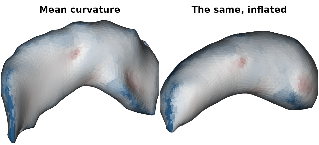

7. Subsetting and extracting

vcg_subset_vertex keeps the vertices a logical selector marks and the faces whose corners all survive:

selector <- mesh$vb[1, ] > 0
half <- vcg_subset_vertex(mesh, selector)
c(input = ncol(mesh$vb), kept = ncol(half$vb))
#> input  kept 
#>  4318  2194

vcg_mesh_patch cuts a mesh along a closed loop of waypoints. They are snapped to the nearest vertices, the loop between them is walked, and the result is a two-element list: the enclosed patch and everything else.

target <- vcg_uniform_remesh(vcg_sphere(), verbose = FALSE)
patches <- vcg_mesh_patch(target, waypoints = diag(1, 3))
vapply(patches, function(p) ncol(p$it), 0L)
#> [1]  931 6517

graphics::par(mar = c(0.1, 0.1, 0.1, 0.1))
plot_mesh_polygon(patches, col = list("#a33a3a", "gray70"),
                  alpha = c(1, 0.55), eye = c(10, 10, 10), zoom = 1.2,
                  shadow_color = "white", ambient_intensity = 0.55)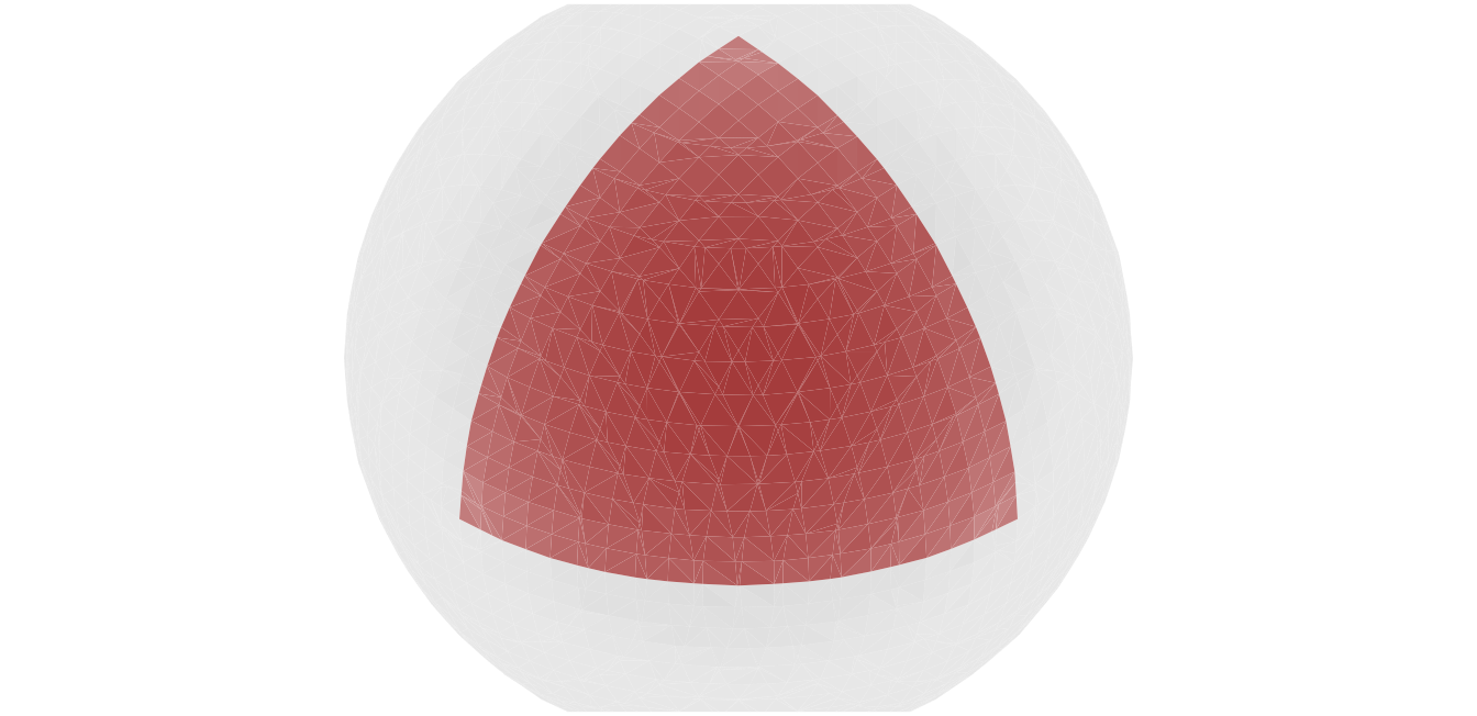

dijkstras_surface_distance walks the mesh graph from a start vertex and returns the geodesic distance to every other vertex; surface_path then reads the shortest path to any target back out of that result. Note that it takes the transposed matrices – one row per vertex and one row per face:

dist <- dijkstras_surface_distance(
  positions = t(mesh$vb[1:3, ]),
  faces = t(mesh$it),
  start_node = 1,
  face_index_start = 1
)
path <- surface_path(dist, target_node = ncol(mesh$vb))
c(vertices_on_path = length(path$path), length = max(path$distance))
#> vertices_on_path           length 
#>         61.00000         61.72654

Because the walk follows edges, the answer depends on the sampling – which is the practical reason to run mris_remesh before measuring distances across a surface.

8. Drawing

plot_mesh_polygon projects every triangle with an orthographic camera, shades it by how directly it faces that camera, depth-sorts everything, and draws it in a single polygon call. plot_mesh_dotcloud draws vertices as rim-lit dots instead. plot() dispatches to whichever suits the mesh.

Both take a list of meshes and render them into one shared depth space, so several surfaces compose correctly. For one mesh, col is a single color, a character vector of one color per vertex, or any other vector, which is read as a depth gradient; for a list of meshes, pass a list of those, one element per mesh. alpha is one value per mesh. A mesh with no face matrix is drawn as one small vcg_sphere per vertex, scaled by cex – which is how the ray hits in section 2 were rendered.

Two controls are worth knowing. mesh_clipping discards triangles whose normal points along the camera ray, peeling the front cap off a closed surface; pair it with side = "both" so the exposed back wall is drawn rather than culled in turn. clipping_plane culls faces against arbitrary world-space planes instead – each a length-5 vector of a normal, a signed offset, and which half-space to keep – and clipping_plane_enabled exempts individual meshes from it, which is how electrodes stay whole while the surface around them is cut away.

Scattering some probes inside the surface – found with the same interior test from section 2 – shows why the exemption matters: cut the surface open and the probes stay whole.

bbox <- apply(fs_style$vb[1:3, ], 1L, range)
set.seed(1)
candidates <- cbind(
  stats::runif(600, bbox[1, 1], bbox[2, 1]),
  stats::runif(600, bbox[1, 2], bbox[2, 2]),
  stats::runif(600, bbox[1, 3], bbox[2, 3])
)
inside <- vcg_detect_collision(fs_style, candidates,
                               include_interior = TRUE)$hit_unit %in% TRUE
probes <- structure(
  list(vb = t(candidates[inside, , drop = FALSE])),
  class = "mesh3d"
)
sum(inside)
#> [1] 74

eye <- c(0, 100, 30)
graphics::par(mfrow = c(1, 3), mar = c(0.1, 0.1, 2.1, 0.1), cex.main = 0.95)

plot_mesh_polygon(fs_style, col = "steelblue", eye = eye, up = c(0, 0, 1),
                  zoom = 1.1, main = "Whole surface")

plot_mesh_polygon(
  list(fs_style, probes),
  col = list("steelblue", "#a33a3a"), cex = 1.1,
  eye = eye, up = c(0, 0, 1), zoom = 1.1,
  clipping_plane = c(0, 1, 0, 0, -1),
  clipping_plane_enabled = c(TRUE, FALSE),
  main = "Cut open, probes exempt"
)

# `plot_mesh_dotcloud` has no `main`; add the title afterwards
plot_mesh_dotcloud(fs_style, col = "steelblue", eye = eye, up = c(0, 0, 1),
                   zoom = 1.1, cex = 0.45)
graphics::title(main = "plot_mesh_dotcloud")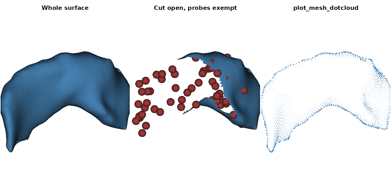

If rgl is installed, rgl_view and rgl_call drive an interactive window using the same meshes, and rgl_plot_normals draws the normal field:

rgl_view({
  rgl_call("shade3d", mesh, col = "steelblue")
  rgl_call("wire3d", mesh, col = "black")
})

References

Botsch, M, and Kobbelt, L (2003). A remeshing approach to multiresolution modeling. Proceedings of the 2004 Eurographics/ACM SIGGRAPH Symposium on Geometry Processing, 185-192.

Fischl, B, Sereno, MI, and Dale, AM (1999). Cortical surface-based analysis II: inflation, flattening, and a surface-based coordinate system. NeuroImage, 9(2), 195-207.

The vcg_* functions are built on vcglib from the Visual Computing Lab, ISTI.