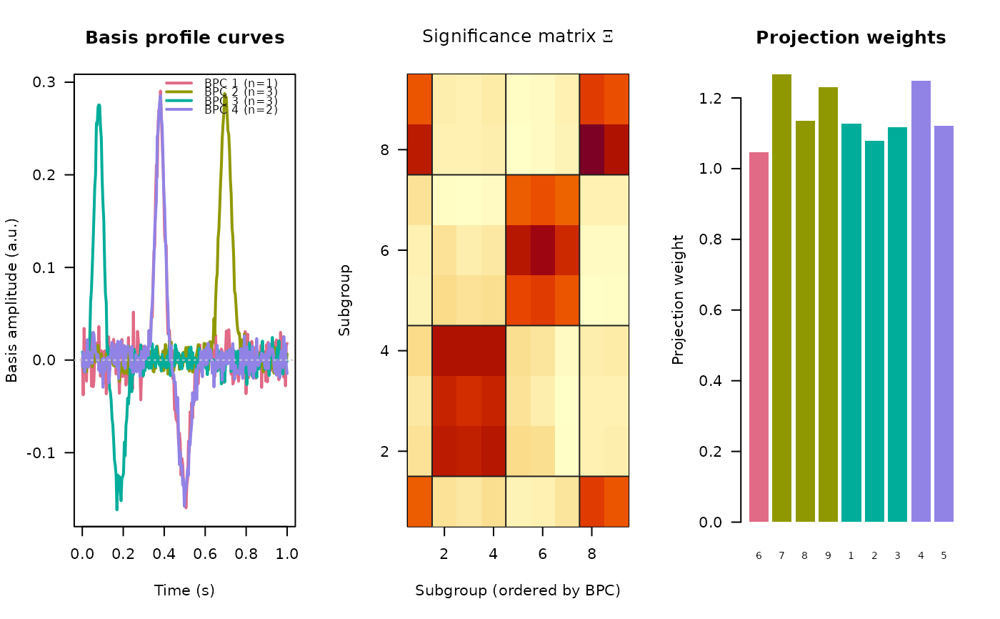
Basis Profile Curve (BPC) identification

Identifies a small set of canonical temporal response shapes - basis profile curves (BPCs) - from the single-trial stimulation-evoked responses recorded at one measurement electrode, where the trials are grouped by stimulation site (or any other condition). Each stimulation group is assigned to the BPC that best explains its trials, and the projection strength of every group is quantified. This is the across-stimulation-site BPC method (see ‘References’); the related crp_cluster applies the same idea across electrodes.

Usage

bpc(
  x,
  groups,
  time = NULL,
  time_window = NULL,
  n_bpc = NULL,
  initial_rank = NULL,
  zeta_threshold = 1,
  null_class = TRUE,
  nmf_max_iters = 10000,
  nmf_tol = c(1e-04, 1e-08),
  verbose = TRUE
)

Arguments

x: numeric matrix of single-trial evoked voltages with shape time x trials (rows are timepoints, columns are trials). All trials across all stimulation groups are stacked column-wise.
groups: vector of length ncol(x) (integer, character or factor) giving the stimulation subgroup of each column of x. At least two subgroups are required and each subgroup needs at least two trials.
time: optional numeric vector of length nrow(x) giving the stimulus-aligned time (in seconds) of each row of x. Only used to crop to time_window and as the plotting axis; the method itself does not require it.
time_window: optional numeric c(lo, hi) analysis window (seconds); requires time. An NA extends to the corresponding data edge. NULL (the default) uses all rows.
n_bpc: integer or NULL; if given, fixes the number of basis curves and skips automatic rank selection.
initial_rank: integer or NULL; the starting NMF rank for automatic selection. NULL uses min(n - 1L, 10L) where \(n\) is the number of subgroups.
zeta_threshold: numeric \(> 0\); rank-selection cutoff on \(\zeta\) (see ‘Details’); smaller values give fewer curves. Defaults to 1, matching the BPC reference.
null_class: logical; if TRUE (the default) subgroups whose winner-take-all loading falls below \(1/(2\sqrt{n})\) are left unassigned (NA); if FALSE every subgroup is forced into a curve.
nmf_max_iters, nmf_tol: passed to naive_nmf.
verbose: logical; whether to report progress.

Value

A named list of class ravetools_bpc:

curves: Numeric matrix, time \(\times\) number of BPCs; column \(q\) is the basis profile curve \(B_q(t)\), the first linear-kernel PCA component of its member trials (unit-norm, sign-oriented to a positive mean projection).
time: Numeric vector, the (windowed) time axis for curves; the sample index when time was not supplied.
group_labels: The unique stimulation subgroup labels, in the order used by clusters and xi.
clusters: Integer vector, the BPC index assigned to each subgroup; NA for subgroups left in the null class.
excluded_groups: The labels of subgroups not represented by any BPC.
weights: A data.frame with one row per (BPC, subgroup) membership: bpc, group, n_trials, weight (mean residual-normalized \(\alpha\)) and p_value.
alpha: Numeric matrix, trials \(\times\) number of BPCs; the per-trial projection \(\alpha\) of every trial onto each basis curve.
xi: Numeric matrix, the \(n \times n\) significance matrix \(\Xi\).
nmf: The naive_nmf result for the selected rank, with H (raw loadings) and H0 (winner-take-all, thresholded).
n_bpc: Integer, the number of basis curves found.
time_window: The effective analysis window used (or NULL).

Details

Let \(V\) be the (windowed) \(T \times K\) matrix of all single trials and let groups map each of the \(K\) columns to one of \(n\) stimulation subgroups.

Window. When time and time_window are supplied the rows of x are cropped to that window; otherwise all rows are used. Rows with non-finite values are dropped.
Internal projections. Each trial is \(L_2\)-normalized into \(V_0\), and \(P = V_0^\top V\) collects the projection of every native trial onto every normalized trial.
Significance matrix. For each ordered pair of subgroups \((k, l)\) the set of relevant entries of \(P\) is gathered (the off-diagonal of the within-group block when \(k = l\), the whole cross block otherwise) and reduced to a one-sample t-statistic versus zero. These form the \(n \times n\) significance matrix \(\Xi\).
Rank selection. \(\Xi\) is made non-negative and rescaled, then factorized with naive_nmf at decreasing inner rank while the degeneracy score \(\zeta\) - the sum of the upper off-diagonal of the row-normalized \(HH^\top\) - exceeds zeta_threshold.
Assignment. Each subgroup takes its winner-take-all BPC over the normalized NMF loadings; with null_class, loadings below \(1/(2\sqrt{n})\) are left unassigned (the “null” class).
Basis curves. Per BPC, the first linear-kernel PCA component of all trials in its member subgroups, sign-oriented to a positive mean projection.
Weights. For each member subgroup the per-trial coefficient \(\alpha\) (projection onto the basis curve) is normalized by the residual magnitude; the mean is the projection weight and a one-sample t-test gives a significance value.

References

The BPC method is described in doi:10.1371/journal.pcbi.1008710 , with a reference Python implementation at https://github.com/MultimodalNeuroimagingLab/bpc_jupyter.

Examples

# Three response shapes, several stimulation groups per shape.
# \donttest{
set.seed(1)
n_time <- 300L
tt <- seq(-0.2, 1, length.out = n_time)
shapes <- list(
  exp(-((tt - 0.08) / 0.03)^2) - 0.5 * exp(-((tt - 0.18) / 0.04)^2),
  exp(-((tt - 0.38) / 0.03)^2) - 0.5 * exp(-((tt - 0.50) / 0.04)^2),
  exp(-((tt - 0.70) / 0.04)^2)
)

# 3 stimulation groups per shape, 12 trials each
V <- NULL
groups <- NULL
g <- 0L
for (s in seq_along(shapes)) {
  for (rep in seq_len(3L)) {
    g <- g + 1L
    trials <- outer(shapes[[s]], runif(12L, 0.5, 1.5)) +
      matrix(rnorm(n_time * 12L, sd = 0.2), n_time, 12L)
    V <- cbind(V, trials)
    groups <- c(groups, rep(g, 12L))
  }
}

res <- bpc(V, groups, time = tt, time_window = c(0, 1), verbose = TRUE)
#> rank 8: HH^T off-diagonal sum = 7.523 > 1.00, reducing
#> rank 7: HH^T off-diagonal sum = 5.148 > 1.00, reducing
#> rank 6: HH^T off-diagonal sum = 3.754 > 1.00, reducing
#> rank 5: HH^T off-diagonal sum = 2.788 > 1.00, reducing
#> selected rank 4 (HH^T off-diagonal sum = 0.667)
res$n_bpc
#> [1] 4
res$clusters
#> [1] 3 3 3 4 4 1 2 2 2
plot(res)

# }

Basis Profile Curve (`BPC`) identification