Canonical Response Parameterization (CRP)

Parameterizes single-trial evoked responses (e.g. cortico-cortical evoked potentials, CCEPs) using the Canonical Response Parameterization method (see 'Citation'). The function estimates the response duration $\tau_R$, the time after stimulus at which the evoked response has its most consistent, shared structure across trials. The estimator is obtained from the time course of cross-trial projection magnitudes, extracts the canonical response shape $C(t)$ via a linear kernel-trick PCA on the trial matrix truncated at $\tau_R$, and reports per-trial weights, residuals, signal-to-noise, explained variance and extraction-significance statistics.

This is an R translation of CRP_method.m (and the surrounding artifact-rejection / duration-uncertainty logic in CRP_illustration.m) from the upstream MATLAB reference implementation; see ‘References’.

Usage

crp(
  x,
  time,
  t_start = 0.015,
  t_end = 1,
  remove_artifacts = TRUE,
  artifact_interval = c("full", "tR"),
  artifact_p_threshold = 1e-05,
  threshold_quantile = 0.98,
  time_step = 5L,
  detect_onset = FALSE,
  onset_search_start = NULL
)

Arguments

x: numeric matrix of single-trial evoked voltages with shape time x trials (i.e. rows are timepoints, columns are trials); the matrix orientation matches the variable V / data in the MATLAB reference. At least two trials are required.
time: numeric vector of length nrow(x) giving the stimulus-aligned time (in seconds) of each row of x; must be monotonically increasing and span [t_start, t_end].
t_start, t_end: numeric scalars, post-stimulation start and end times (in seconds) defining the analysis window. Defaults match the MATLAB illustration (0.015 s to 1 s).
remove_artifacts: logical; if TRUE (the default), an initial CRP pass is run to identify outlier/artifact trials, which are then dropped before the final pass. See ‘Details’.
artifact_interval: character, one of "full" (the default, matching the active option in the MATLAB illustration) or "tR"; selects whether per-trial outlier statistics are computed on the projection magnitudes for the full window or only at the response duration $\tau_R$.
artifact_p_threshold: numeric, p-value threshold below which a trial is flagged as artifact (provided its mean projection is also below the cohort mean); defaults to 1e-5.
threshold_quantile: numeric in (0, 1); the fraction of the peak mean projection magnitude used to derive the duration-uncertainty bounds tau_R_lower and tau_R_upper. Defaults to 0.98 as in the manuscript.
time_step: integer, sampling step (in samples) used when sweeping candidate response duration; defaults to 5L, matching the MATLAB t_step. Larger values are faster but smooth the projection profile.
detect_onset: logical; if TRUE, estimate the response onset $\tau_{onset}$ via a reverse cumulative-projection scan (see ‘Details’). The forward canonical shape and per-trial weights are left unchanged; only the reported canonical shape C is restricted to the active response support $[\tau_{onset}, \tau_R]$. The onset may fall before t_start (down to onset_search_start). Defaults to FALSE.
onset_search_start: numeric scalar or NULL; the earliest time (in seconds) the onset scan may reach when detect_onset = TRUE. NULL (the default) uses the first loaded time point, so the scan can look across the entire signal before $\tau_R$. Raise it to keep the scan away from an early stimulation artifact. Clamped into [min(time), t_end].

Value

A named list with the following elements:

parameters

A list of single-trial parameterizations (crp_parms in MATLAB):

C: Numeric vector, the reported canonical response shape $C(t)$, taken as the slice of C_full over its active support (so it shares identical values with C_full). By default this is $[t_{start}, \tau_R]$, where it equals the first eigenvector of the linear kernel PCA on V_tR (oriented to the mean trace, unit-norm, length $T_R$). When detect_onset = TRUE it is restricted to $[\tau_{onset}, \tau_R]$ (so its norm is then $\le 1$). The matching time axis is params_times.
C_full: Numeric vector spanning the entire loaded time range (every row of time, including any baseline at $t < 0$). Obtained by applying the trial-space loading to the full retained data, so C_full coincides exactly with the untrimmed forward C on $[t_{start}, \tau_R]$ and extrapolates the shape everywhere else. Time axis is params_times_full. Outside $[t_{start}, \tau_R]$ cross-trial consistency is not optimized, so those portions are more variable.
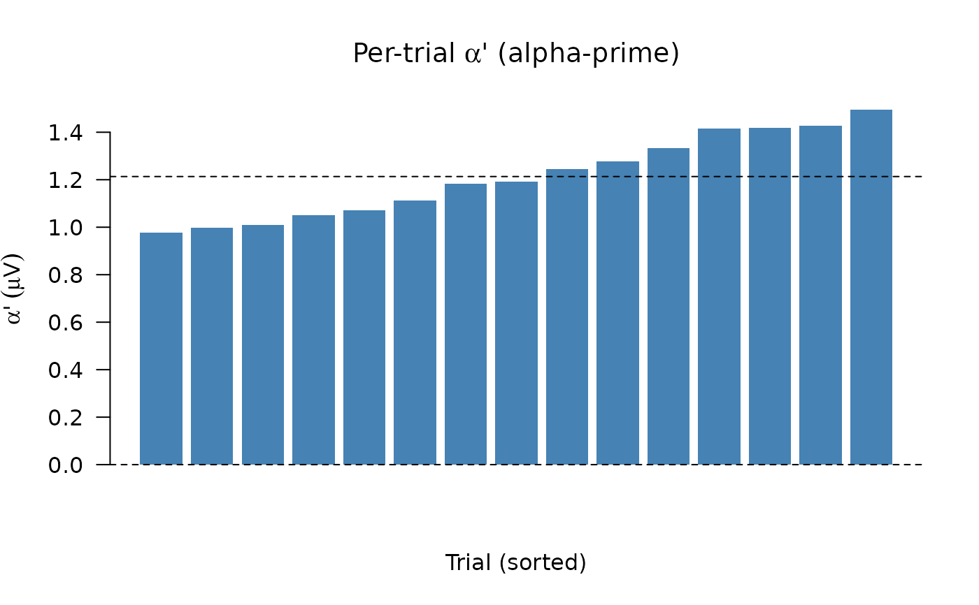
loading: Numeric vector of length $K$ (retained trials), the trial-space loading $g = V_{tR}^\top C = s_1 v_1$ recovered from the forward decomposition. Applying it to a time $\times$ trials matrix and dividing by $\|g\|^2$ reconstructs the canonical shape over that time range; this is how C_full is formed.
al: Numeric vector of length $K$ (number of trials), the per-trial alpha coefficient $\alpha_k = C^\top V_k$: scalar projection of trial $k$ onto $C(t)$. Larger magnitude means the trial resembles the canonical shape more strongly; sign reflects polarity relative to $C$.
al_p: Numeric vector of length $K$, alpha-prime $\alpha_k / \sqrt{T_R}$: al rescaled to remove the duration dependence from the unit-norm convention on $C$. Expressed in $\mu V$ and comparable across electrodes or conditions with different $\tau_R$.
ep: Numeric matrix of shape $T_R \times K$, the per-trial residual $\epsilon_k(t) = V_k(t) - \alpha_k C(t)$ after the shared component is removed, computed over the forward window $[t_{start}, \tau_R]$ against the untrimmed forward canonical shape. Access trial $k$ via ep[, k]. (When detect_onset = TRUE the reported C may be shorter than $T_R$; ep always stays on the full forward window.)
epep_root: Numeric vector of length $K$, $\|\epsilon_k\| = \sqrt{\epsilon_k^\top \epsilon_k}$: L2 norm of the residual per trial. Smaller values indicate the canonical shape describes that trial more faithfully.
Vsnr: Numeric vector of length $K$, per-trial signal-to-noise $\alpha_k / \|\epsilon_k\|$. Values $> 1$ indicate the canonical component is larger than the residual.
expl_var: Numeric vector of length $K$, per-trial explained variance $1 - \|\epsilon_k\|^2 / \|V_k\|^2$: fraction of each trial's energy accounted for by $\alpha_k C(t)$. Ranges in $[0, 1]$.
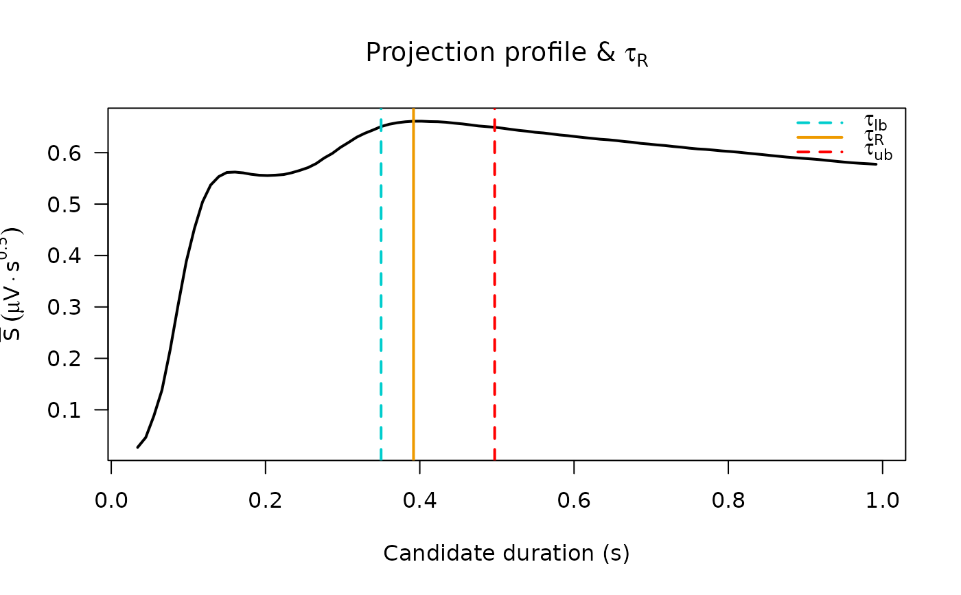
tR: Numeric scalar, response duration $\tau_R$ in seconds: the time at which mean cross-trial projection magnitude is maximized.
params_times: Numeric vector, time axis for the reported C; length matches C ($T_R$, or the onset-trimmed support when detect_onset = TRUE).
params_times_full: Numeric vector, time axis for C_full; equals the full loaded time (every row, including the baseline at $t < 0$).
V_tR: Numeric matrix $T_R \times K$, trial matrix truncated to $\tau_R$ - the data actually decomposed. Together with ep and avg_trace_tR it always spans the full forward window $[t_{start}, \tau_R]$, independently of detect_onset.
avg_trace_tR: Numeric vector of length $T_R$, simple trial average truncated to $\tau_R$.

projections

A list of projection-stage outputs (crp_projs in MATLAB):

proj_tpts: Numeric vector, candidate duration time points (seconds) at which projection magnitudes were evaluated.
S_all: Numeric matrix; rows are non-redundant off-diagonal trial-pair projections, columns correspond to proj_tpts. Units: $\mu V \cdot s^{1/2}$.
mean_proj_profile: Numeric vector, mean of S_all across trial pairs at each candidate duration, the profile whose maximum defines $\tau_R$.
var_proj_profile: Numeric vector, variance of S_all across trial pairs at each candidate duration.
tR_index: Integer, column index into S_all and proj_tpts corresponding to $\tau_R$.
tR_sample: Integer, row (sample) index of $\tau_R$ within the windowed data; V[seq_len(tR_sample), ] is the truncated trial matrix V_tR.
avg_trace_input: Numeric vector, simple trial average over the full analysis window (not truncated to $\tau_R$).
stat_indices: Integer vector, row indices of S_all used for the significance t-tests, constructed so each trial-pair comparison appears at most once.
t_value_tR, p_value_tR: t-statistic and one-sided p-value (H1: mean projection $> 0$) at $\tau_R$. Primary extraction-significance test reported in the manuscript.
t_value_full, p_value_full: Same test at the full analysis-window duration.

bad_trials

Integer vector of column indices into the original x flagged and removed as artifacts; integer(0) when none removed or when remove_artifacts = FALSE.

tau_R

Numeric scalar, estimated response duration $\tau_R$ in seconds (convenience copy of parameters$tR).

tau_R_lower, tau_R_upper

Numeric scalars, lower and upper threshold-crossing times (seconds) bracketing $\tau_R$ at the threshold_quantile fraction of the peak mean projection magnitude.

tau_onset, tau_onset_lower, tau_onset_upper

Numeric scalars, the estimated response onset time (seconds) and its lower/upper threshold-crossing bounds, from the reverse projection scan; all NA unless detect_onset = TRUE.

onset

List with the reverse-scan profile (onset_tpts and mean_proj_profile, mapped onto original time); NULL unless detect_onset = TRUE (also NULL when the search window had too few samples).

t_start, t_end

The analysis window used.

sample_rate

Numeric, sampling rate inferred from time.

Details

Briefly, the algorithm proceeds in three stages:

For a sweep of candidate durations $k$, compute pairwise L2-normalized cross-projection magnitudes between trials truncated to $[0, k]$. The duration that maximizes the mean projection magnitude is taken as the response duration $\tau_R$.
Apply linear kernel-trick PCA to the trial matrix truncated to $\tau_R$; the first principal component is the canonical response shape $C(t)$.
Project $C(t)$ into each trial to obtain per-trial weights $\alpha_k$; the residual $\epsilon_k = V_k - \alpha_k C$ summarizes trial-by-trial deviation from the canonical shape.

Significance is assessed by a one-sided t-test on the off-diagonal projection magnitudes against zero, restricted to a non-overlapping subset of comparison pairs to avoid double-counting.

When remove_artifacts = TRUE, the function performs an initial CRP pass and runs an unpaired t-test for each trial comparing the projections it participates in against all other off-diagonal projections. Trials with p < artifact_p_threshold and mean projection below the cohort mean are dropped, and CRP is re-run.

When detect_onset = TRUE, a complementary reverse pass estimates the response onset. The retained trials between onset_search_start and $\tau_R$ are time-reversed, and the same cumulative cross-projection profile is computed growing backward from $\tau_R$. The backward duration that maximizes cross-trial consistency marks $\tau_{onset}$, the time at which trials begin to share structure - useful when the response is delayed by an unknown latency. Because the scan can extend before t_start, the onset may be earlier than the analysis window. This pass only locates a time: it re-uses the forward loading, so the canonical shape and per-trial weights are unchanged (the reported C is merely sliced to $[\tau_{onset}, \tau_R]$).

Time points whose data are not finite (any NA, NaN or Inf across trials) are dropped before analysis. t_start, t_end and onset_search_start are clamped into the available time range rather than triggering an error.

References

The CRP algorithm is described in doi:10.1371/journal.pcbi.1011105 , with a reference MATLAB implementation at https://github.com/kaijmiller/crp_scripts. See citation("ravetools") for the full bibliographic entry.

Examples

set.seed(42)

# Synthetic CCEP-like data: shared canonical shape with per-trial scaling
n_time   <- 500L
n_trials <- 20L
tt <- seq(-0.5, 1, length.out = n_time)
canonical <- exp(-((tt - 0.10) / 0.05)^2) -
             0.5 * exp(-((tt - 0.30) / 0.10)^2)
V <- (outer(canonical, runif(n_trials, 0.5, 1.5)) +
       matrix(rnorm(n_time * n_trials, sd = 0.3), n_time, n_trials)) * 2

res <- crp(V, tt)

op <- par(mfrow = c(1, 3), mar = c(4.5, 4, 3, 1))
on.exit({ par(op) })

# ---- Panel 1: all trials (full window) + mean + C(t) overlay ----------
parms <- res$parameters
matplot(tt, V, type = "l", lty = 1,
        col = "#80808060", xlab = "Time (s)",
        ylab = expression(mu * V),
        main = expression("Canonical shape " * C(t)))
# scale C(t) to the amplitude of the mean trace for overlay;
# C(t) ends at tau_R so the line is cut off there naturally
C_scaled <- parms$C * max(abs(rowMeans(V))) / max(abs(parms$C))
lines(parms$params_times, C_scaled, col = "#FFFF0080", lwd = 3)

# Mean
lines(tt, rowMeans(V), col = "black", lwd = 1)
legend("topright", c("mean", "C(t) scaled"),
       col = c("black", "#FFFF00"), lty = c(1, 2), lwd = 2,
       bty = "n", cex = 0.8)


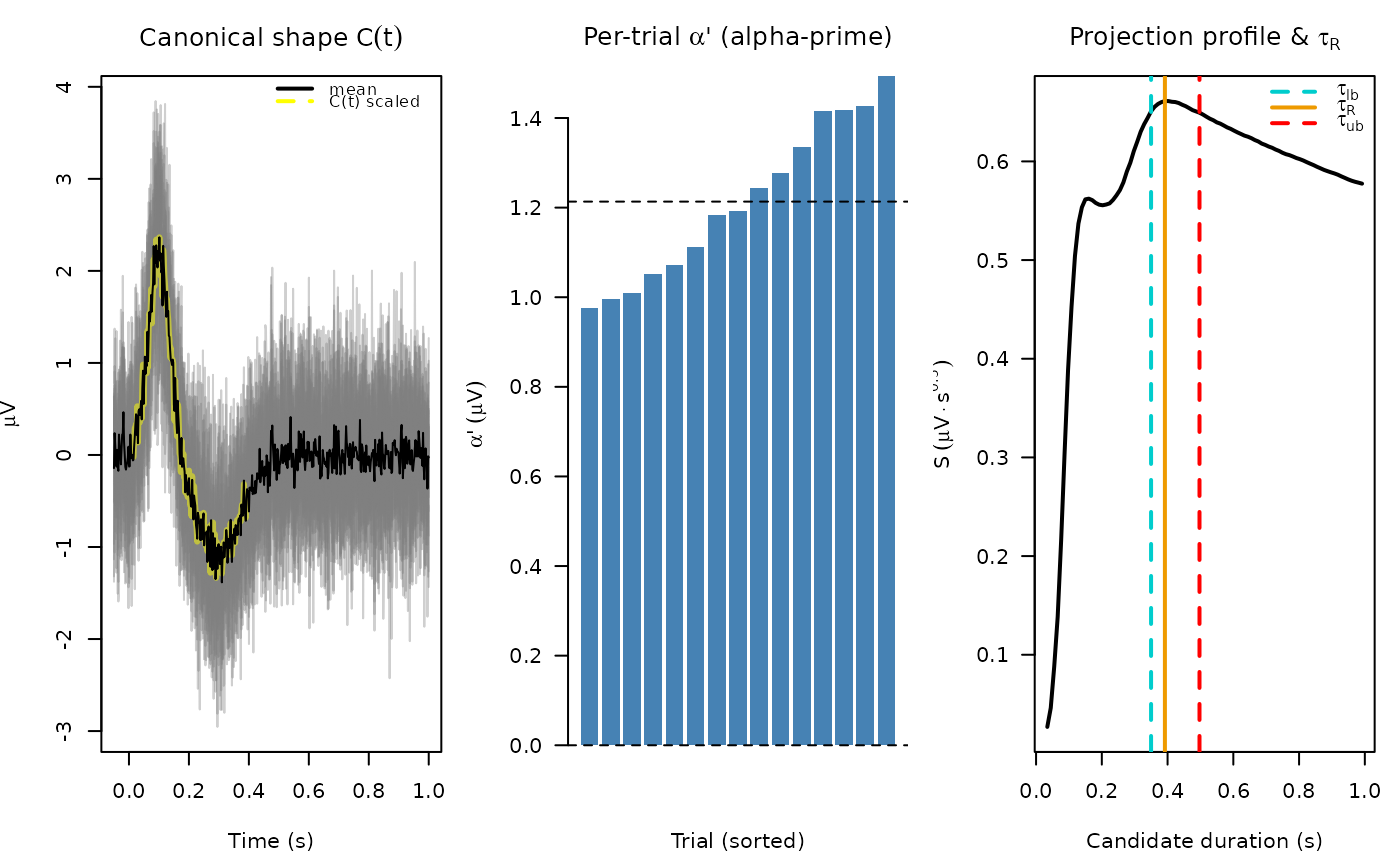# ---- Panel 2: per-trial alpha-prime weights -----------------------------
barplot(sort(parms$al_p), col = "steelblue", border = NA, las = 1,
        xlab = "Trial (sorted)",
        ylab = expression(alpha * "'" ~ (mu * V)),
        main = expression("Per-trial " * alpha * "' (alpha-prime)"))
abline(h = c(0, mean(parms$al_p)), lty = 2)


# ---- Panel 3: mean projection profile with tau_R bounds ----------------
proj <- res$projections
plot(proj$proj_tpts, proj$mean_proj_profile, type = "l", lwd = 2,
     xlab = "Candidate duration (s)",
     ylab = expression(bar(S) ~ (mu * V %.% s^{0.5})),
     main = expression("Projection profile & " * tau[R]),
     las = 1)
abline(v = c(res$tau_R_lower, res$tau_R, res$tau_R_upper),
       col = c("cyan3", "orange2", "red"),
       lty = c(2, 1, 2), lwd = 2)
legend("topright",
       legend = expression(tau[lb], tau[R], tau[ub]),
       col = c("cyan3", "orange2", "red"),
       lty = c(2, 1, 2), lwd = 2, bty = "n")


par(op)

# ---- Onset detection (reverse scan) on the same data -------------------
res_onset <- crp(V, tt, detect_onset = TRUE)
c(tau_onset = res_onset$tau_onset, tau_R = res_onset$tau_R)
#>  tau_onset      tau_R 
#> 0.03206413 0.37474950