ieegio supports reading from and writing to multiple
imaging formats:
- Volume:
NIfTI&FreeSurfer MGH/MGZ - Surface:
GIfTI&FreeSurfergeometry, annotation, curvature/measurement,wformat,AFNI/SUMANIML,VTKpolygon meshes - Streamlines:
TRK,TCK,TT(read-only),VTK,VTP, …
Beyond reading and writing, ieegio can also map data
between volumes and surfaces, chain coordinate transforms, and compare
regions of interest; those are covered at the end of this article.
To start, please load ieegio. This vignette uses sample
data which requires extra download.
library(ieegio)

# volume file
nifti_file <- ieegio_sample_data("brain.demosubject.nii.gz")

# geometry
geom_file <- ieegio_sample_data(
  "gifti/icosahedron3d/geometry.gii")

# measurements
shape_file <- ieegio_sample_data(
  "gifti/icosahedron3d/rand.gii"
)

# time series
ts_file <- ieegio_sample_data(
  "gifti/icosahedron3d/ts.gii")

# streamlines
trk_file <- ieegio_sample_data(
  "streamlines/CNVII_R.trk")

tck_file <- ieegio_sample_data(
  "streamlines/CNVII_R.tck")

tt_file <- ieegio_sample_data(
  "streamlines/CNVII_R.tt")

# AFNI/SUMA std.141 geometry and matching annotation
std141_geom_file <- ieegio_sample_data(
  "gifti/std.141.lh.inf_200.gii")

niml_file <- ieegio_sample_data(
  "niml/std.141.lh.aparc.a2009s.annot.niml.dset")

# volumetric atlas
atlas_file <- ieegio_sample_data(
  "atlases/YBA/YBA690.nii.gz")
Volume files
ieegio::read_volume and
ieegio::write_volume provides high-level interfaces for
reading and writing volume data such as MRI,
CT. fMRI, etc.
Each volume data (NIfTI, MGH, …) contains a
header, a data, and a transforms
list.
volume <- read_volume(nifti_file)
volume
#> <Image Volume>
#>   Type : rnifti/nifti
#>   Shape: c(256L, 256L, 256L)
#>   Transforms:
#>     vox2ras:
#>       [-1   0  0   131.6]
#>       [ 0   0  1  -127.5]
#>       [ 0  -1  0   127.5]
#>       [ 0   0  0       1]
#>     vox2ras_tkr:
#>       [-1   0  0   128]
#>       [ 0   0  1  -128]
#>       [ 0  -1  0   128]
#>       [ 0   0  0     1]
#>     vox2fsl:
#>       [1  0  0  0]
#>       [0  1  0  0]
#>       [0  0  1  0]
#>       [0  0  0  1]
The transforms contain transforms from volume (column, row, slice)
index to other coordinate systems. The most commonly used one is
vox2ras, which is a 4x4 matrix mapping the
voxels to scanner (usually T1-weighted) RAS
(right-anterior-superior) system.
Accessing the image values via [ operator. For
example,
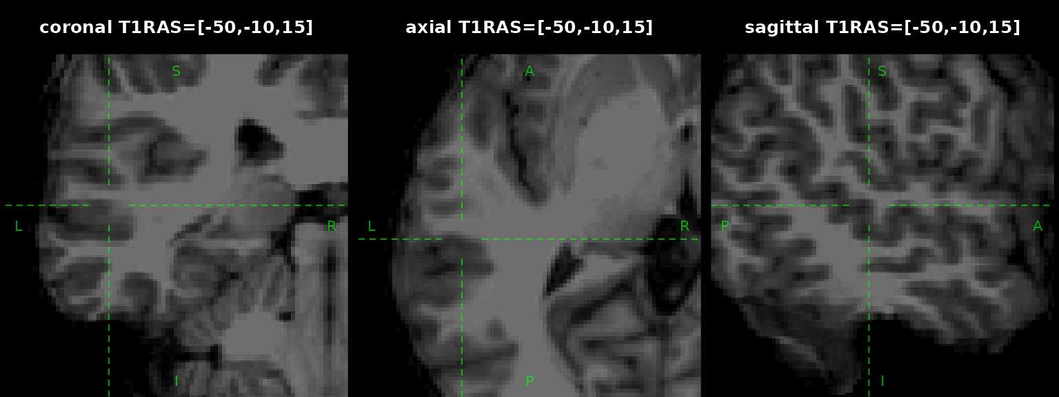
volume[128, , ]Plotting the anatomical slices:
par(mfrow = c(1, 3), mar = c(0, 0, 3.1, 0))

ras_position <- c(-50, -10, 15)

ras_str <- paste(sprintf("%.0f", ras_position), collapse = ",")

for (which in c("coronal", "axial", "sagittal")) {
  plot(x = volume, position = ras_position, crosshair_gap = 10,
       crosshair_lty = 2, zoom = 3, which = which,
       main = sprintf("%s T1RAS=[%s]", which, ras_str))
}
Surface files
Reading surface file using read_surface supports
multiple data types
library(ieegio)
# geometry
geometry <- read_surface(geom_file)

# measurements
measurement <- read_surface(shape_file)

# time series
time_series <- read_surface(ts_file)
You can merge them to a single object, making an object with multiple embedding data-sets:
merged <- merge(geometry, measurement, time_series)
#> Merging geometry attributes, assuming all the surface objects have the same number of vertices.
print(merged)
#> <ieegio Surface>
#>   Header class: basic_geometry
#>   Geometry :
#>     # of Vertex     : 12
#>     # of Face index : 20
#>     # of transforms : 1
#>       Transform Targets : Unknown
#>   Measurements: `Shape001`
#>   Time series:
#>     # of time points: 4
#>     Average slice duration: 1
#>
#> Contains: `geometry`, `measurements`, `time_series`
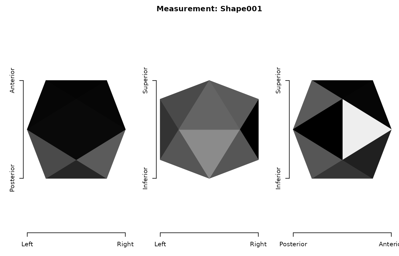
Plot the surfaces in 3D viewer, colored by shape
measurement
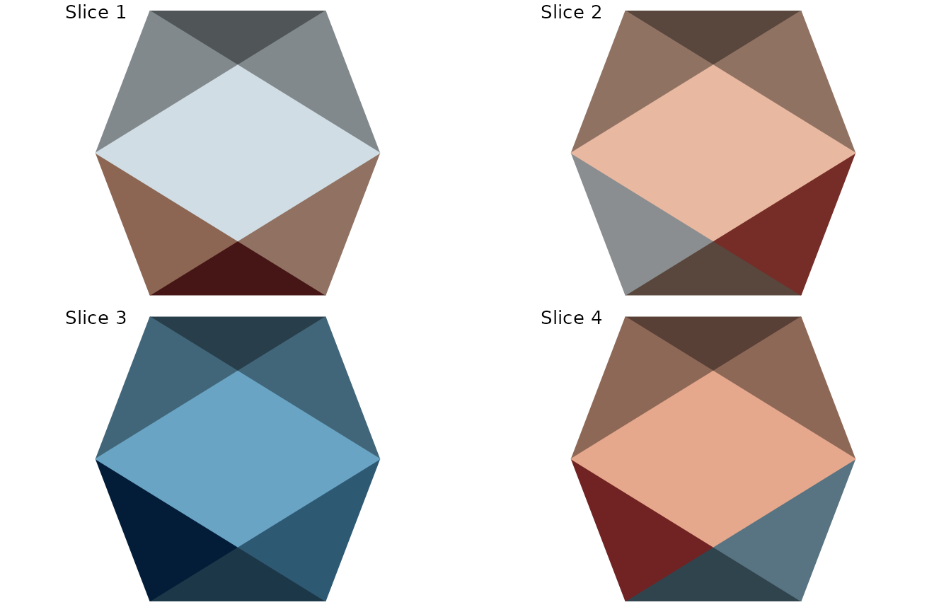
Plot the normalized time-series data
ts_demean <- apply(
  merged$time_series$value,
  MARGIN = 1L,
  FUN = function(x) {
    x - mean(x)
  }
)
merged$time_series$value <- t(ts_demean)
plot(
  merged, name = "time_series",
  col = c(
    "#053061", "#2166ac", "#4393c3",
    "#92c5de", "#d1e5f0", "#ffffff",
    "#fddbc7", "#f4a582", "#d6604d",
    "#b2182b", "#67001f"
  )
)
Streamline files
Reading streamlines via universal entry function
read_streamlines
trk <- read_streamlines(trk_file, half_voxel_offset = TRUE)
tck <- read_streamlines(tck_file)
tt <- read_streamlines(tt_file)
To obtain the streamline data
message("Total number of streamlines: ", length(trk))
#> Total number of streamlines: 54

head(trk[[1]]$coords)
#>          [,1]      [,2]      [,3]
#> [1,] 37.81250 -26.12500 -34.87500
#> [2,] 37.37500 -26.28125 -34.96875
#> [3,] 36.90625 -26.43750 -35.06250
#> [4,] 36.43750 -26.62500 -35.18750
#> [5,] 35.96875 -26.78125 -35.28125
#> [6,] 35.53125 -26.93750 -35.37500
To preview the streamline data
pal <- colorRampPalette(c("navy", "grey", "red"))
plot(trk, col = pal(length(trk)))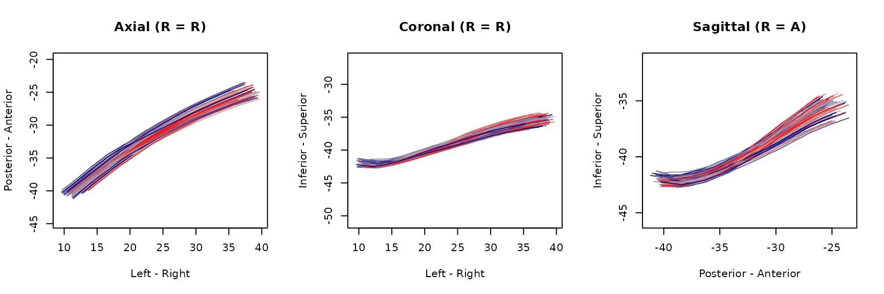
To write the streamlines, for example, write tck file to
trk file:
# Create a temporary file
tfile <- tempfile(fileext = ".trk")
write_streamlines(x = tck, con = tfile)
Surface annotations from AFNI/SUMA
NIML datasets (file names ending with
.niml.dset) are read by the same read_surface
entry point. The data type is resolved from the dataset itself: datasets
carrying a label table are read as annotations, the rest as
measurements.
std141_geometry <- read_surface(std141_geom_file)

annotation <- read_surface(niml_file)
annotation
#> <ieegio Surface>
#>   Header class: niml_dset
#>   Annotations: `node label`
#>     # of labels: 76
#>
#> Contains: `annotations`
The sample geometry and annotation live on the same
std.141 mesh, so they merge directly:
labeled <- merge(std141_geometry, annotation)
#> Merging geometry attributes, assuming all the surface objects have the same number of vertices.
labeled
#> <ieegio Surface>
#>   Header class: basic_geometry
#>   Geometry :
#>     # of Vertex     : 198812
#>     # of Face index : 397620
#>     # of transforms : 1
#>       Transform Targets : Unknown
#>   Annotations: `node label`
#>     # of labels: 76
#>
#> Contains: `geometry`, `annotations`
plot(labeled, name = "annotations")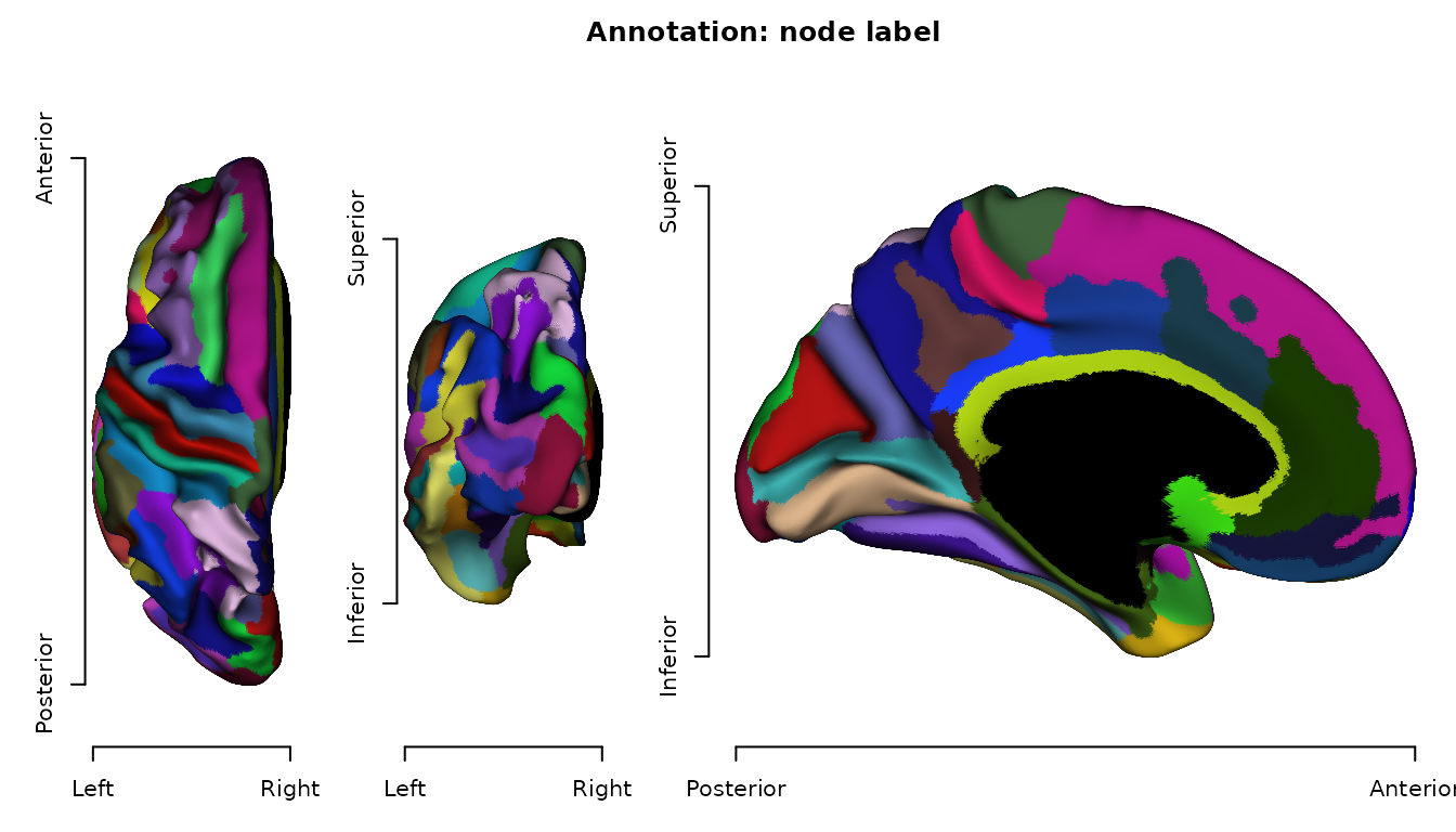
If you need the raw NIML element tree rather than a
surface object, use the low-level io_read_niml together
with niml_find.
Regions of interest
A region of interest is described first and computed later.
as_ieegio_roi records the criteria without applying them,
and resolve_roi_as carries them out, returning geometry in
world (RAS) coordinates.
atlas <- read_volume(atlas_file)

# describe: which voxels count as the region
roi <- as_ieegio_roi(atlas, threshold_lb = 1, threshold_ub = 5)
roi
#> <ieegio ROI [volume]: lower bound 1, upper bound 5>
#> <Image Volume>
#>   Type : rnifti/nifti
#>   Shape: c(197L, 233L, 189L)
#>   Transforms:
#>     vox2ras:
#>       [1  0  0   -98]
#>       [0  1  0  -134]
#>       [0  0  1   -72]
#>       [0  0  0     1]
#>     vox2ras_tkr:
#>       [1  0  0   -98.5]
#>       [0  1  0  -116.5]
#>       [0  0  1   -94.5]
#>       [0  0  0       1]
#>     vox2fsl:
#>       [-1  0  0  196]
#>       [ 0  1  0    0]
#>       [ 0  0  1    0]
#>       [ 0  0  0    1]
# compute: turn that description into geometry
resolve_roi_as(roi, "pointcloud")
#> <ieegio ROI [pointcloud]>
#> <ieegio Surface>
#>   Header class: basic_geometry
#>   Geometry :
#>     # of Vertex     : 3495
#>     # of Face index : 0
#>     # of transforms : 0
#>       Transform Targets :
#>
#> Contains: `geometry`
Because both sides are resolved to world coordinates first, regions stored in different ways can be compared directly. Here the whole atlas is tested against the facial-nerve tracts read earlier:
overlap <- detect_roi_overlap(
  as_ieegio_roi(atlas, threshold_lb = 1),
  trk,
  radius = 2
)
overlap
#> <ieegio ROI overlap: `x` and `y` overlap>
#>   x: volume
#>   y: streamlines (annotated)
#>   Units of `y` overlapping `x`: 53.7%
#>   Early stop: FALSE
The result carries the annotated streamlines back in
overlap$annotated, so each tract knows whether it reached
the region, and overlap$hit_ratio reports the proportion
that did.
Volume to surface
volume_to_surface turns a mask or a set of atlas labels
into a smoothed mesh:
volume_to_surface(atlas, threshold_lb = 1, threshold_ub = 5)
#> <ieegio Surface>
#>   Header class: basic_geometry
#>   Geometry :
#>     # of Vertex     : 1940
#>     # of Face index : 3878
#>     # of transforms : 1
#>       Transform Targets : ScannerAnat
#>
#> Contains: `geometry`
Coordinate spaces and transforms
new_space names a coordinate space, and
surface_to_surface moves a surface into it, recording the
target on the surface transform list.
mni <- new_space("MNI152", orientation = "RAS")
mni
#> MNI152 (RAS)

surface_to_surface(
  geometry,
  space_from = "scanner",
  space_to = mni,
  transform = diag(1, 4)
)
#> <ieegio Surface>
#>   Header class: gifti
#>   Geometry :
#>     # of Vertex     : 12
#>     # of Face index : 20
#>     # of transforms : 1
#>       Transform Targets : MNI152
#>
#> Contains: `geometry`
Transforms themselves can come from other tools:
io_read_ants_transform reads ANTs affine and
displacement field transforms, io_read_flirt_transform
reads FSL FLIRT matrices, and
transform_flirt2ras converts a FLIRT transform
into world (RAS) coordinates.