Show channel signals with diagnostic plots

The diagnostic plots include 'Welch Periodogram' (pwelch) and histogram (hist)

Usage

diagnose_channel(
  s1,
  s2 = NULL,
  sc = NULL,
  srate,
  name = "",
  try_compress = TRUE,
  max_freq = 300,
  window = ceiling(srate * 2),
  noverlap = window/2,
  std = 3,
  which = NULL,
  main = "Channel Inspection",
  col = c("black", "red"),
  cex = 1.2,
  cex.lab = 1,
  lwd = 0.5,
  plim = NULL,
  nclass = 100,
  start_time = 0,
  boundary = NULL,
  mar = c(3.1, 4.1, 2.1, 0.8) * (0.25 + cex * 0.75) + 0.1,
  mgp = cex * c(2, 0.5, 0),
  xaxs = "i",
  yaxs = "i",
  xline = 1.66 * cex,
  yline = 2.66 * cex,
  tck = -0.005 * (3 + cex),
  ...
)

Arguments

s1

the main signal to draw

s2

the comparing signal to draw; usually s1 after some filters; must be in the same sampling rate with s1; can be NULL

sc

decimated s1 to show if srate is too high; will be automatically generated if NULL

srate

sampling rate

name

name of s1, or a vector of two names of s1 and s2 if s2 is provided

try_compress

whether try to compress (decimate) s1 if srate is too high for performance concerns

max_freq

the maximum frequency to display in 'Welch Periodograms'

window, noverlap

see pwelch

std

the standard deviation of the channel signals used to determine boundary; default is plus-minus 3 standard deviation

which

NULL or integer from 1 to 4; if NULL, all plots will be displayed; otherwise only the subplot will be displayed

main

the title of the signal plot

col

colors of s1 and s2

cex, lwd, mar, cex.lab, mgp, xaxs, yaxs, tck, ...

graphical parameters; see par

plim

the y-axis limit to draw in 'Welch Periodograms'

nclass

number of classes to show in histogram (hist)

start_time

the starting time of channel (will only be used to draw signals)

boundary

a red boundary to show in channel plot; default is to be automatically determined by std

xline, yline

distance of axis labels towards ticks

Value

A list of boundary and y-axis limit used to draw the channel

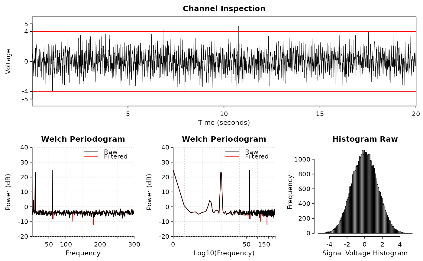
Examples

library(ravetools)

# Generate 20 second data at 2000 Hz
time <- seq(0, 20, by = 1 / 2000)
signal <- sin( 120 * pi * time) +
  sin(time * 20*pi) +
  exp(-time^2) *
  cos(time * 10*pi) +
  rnorm(length(time))

signal2 <- notch_filter(signal, 2000)

diagnose_channel(signal, signal2, srate = 2000,
                 name = c("Raw", "Filtered"), cex = 1)