Convolution of 1D, 2D, 3D data via FFT

Use the 'Fast-Fourier' transform to compute the convolutions of two data with zero padding.

Usage

convolve_signal(x, filter)

convolve_image(x, filter)

convolve_volume(x, filter)

Arguments

x

one-dimensional signal vector, two-dimensional image, or three-dimensional volume; numeric or complex

filter

kernel with the same number of dimensions as x

Value

Convolution results with the same length and dimensions as x. If x is complex, results will be complex, otherwise results will be real numbers.

Details

This implementation uses 'Fast-Fourier' transform to perform 1D, 2D, or 3D convolution. Compared to implementations using original mathematical definition of convolution, this approach is much faster, especially for image and volume convolutions.

The input x is zero-padded beyond edges. This is most common in image or volume convolution, but less optimal for periodic one-dimensional signals. Please use other implementations if non-zero padding is needed.

The convolution results might be different to the ground truth by a precision error, usually at 1e-13 level, depending on the 'FFTW3' library precision and implementation.

Examples

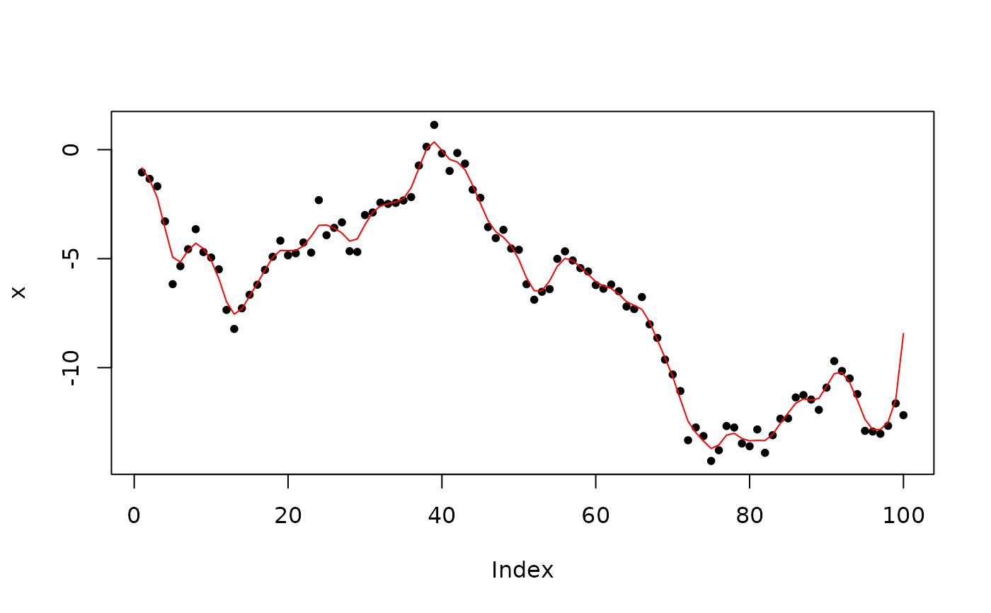
# ---- 1D convolution ------------------------------------
x <- cumsum(rnorm(100))
filter <- dnorm(-2:2)
# normalize
filter <- filter / sum(filter)
smoothed <- convolve_signal(x, filter)

plot(x, pch = 20)
lines(smoothed, col = 'red')


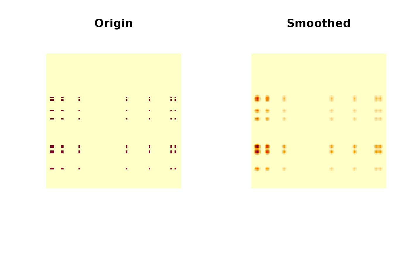
# ---- 2D convolution ------------------------------------
x <- array(0, c(100, 100))
x[
  floor(runif(10, min = 1, max = 100)),
  floor(runif(10, min = 1, max = 100))
] <- 1

# smooth
kernel <- outer(dnorm(-2:2), dnorm(-2:2), FUN = "*")
kernel <- kernel / sum(kernel)

y <- convolve_image(x, kernel)

par(mfrow = c(1,2))
image(x, asp = 1, axes = FALSE, main = "Origin")
image(y, asp = 1, axes = FALSE, main = "Smoothed")