Catmull-Rom 3D Spline Curve

Creates a smooth Catmull-Rom spline curve through a set of 3D key points.

Usage

catmull_rom_3d(
  points,
  curve_type = c("centripetal", "chordal", "uniform"),
  tension = 0.5,
  closed = FALSE
)

Arguments

points

numeric matrix with at least 2 rows and exactly 3 columns (x, y, z), giving the key (control) points through which the curve passes.

curve_type

character; One of "centripetal" (default), "chordal", or "uniform". "centripetal" uses \(\alpha = 0.5\) (square-root of chord length), "chordal" uses \(\alpha = 1\) (chord length), and "uniform" is the classic formulation controlled by tension.

tension

numeric scalar in \([0, 1]\); tangent scaling factor used only when curve_type = "uniform". At 0.5 (default) the curve matches the standard Catmull-Rom formulation.

closed

logical; if TRUE the curve closes on itself by connecting the last point back to the first. Default is FALSE.

Value

An object of class "ravetools_curve" (a list) with the following elements:

points

The input key-point matrix (\(n \times 3\)).

curve_type

Character, the parameterization type.

tension

Numeric, the tension value (relevant for "uniform" only).

closed

Logical, whether the curve is closed.

get_point

A function(t) that accepts a scalar t in \([0, 1]\) and returns a named numeric vector on the curve.

get_points

A function(n) that returns an \(n \times 3\) matrix of n evenly spaced points along the curve, with column names "x", "y", "z".

get_closest_t

A function(query, coarse_n = 200L) that, given a 3-element numeric vector query (x, y, z), returns a list with elements t (the parameter value in \([0, 1]\) of the nearest point), point (the closest point on the curve as a named numeric vector), and distance (Euclidean distance from query to the curve). The search uses coarse_n uniform samples for an initial bracket followed by scalar optimization.

t_keypoints

Numeric vector of length \(n\) with the t parameter value where each key point lies on the curve. First element is always 0, last is always 1.

segment_lengths

Numeric vector of length \(n-1\) (open curve) or \(n\) (closed curve) containing the arc length of each spline segment, estimated by numerical integration.

See also

print.ravetools_curve, plot.ravetools_curve

Examples

pts <- matrix(c(
  -33.0534, -10.6213, -21.8328,
  -34.7526, -25.5089, -14.5390,
  -41.2002, -10.4606, -22.0032,
  -46.4717, -10.3567, -22.1134,
  -51.7431, -10.2528, -22.2237,
  -57.0146, -10.1488, -22.3339,
  -62.2860, -10.0449, -22.4442,
  -67.5575,  -9.9410, -22.5544
), ncol = 3, byrow = TRUE)

curve <- catmull_rom_3d(pts)
print(curve)
#> <ravetools_curve: 8 key points, type=centripetal>
#> Key points (t / x / y / z / seg_length):
#>           t        x        y        z seg_length
#> 1 0.0000000 -33.0534 -10.6213 -21.8328  16.827854
#> 2 0.1428571 -34.7526 -25.5089 -14.5390  18.227558
#> 3 0.2857143 -41.2002 -10.4606 -22.0032   5.400490
#> 4 0.4285714 -46.4717 -10.3567 -22.1134   5.273577
#> 5 0.5714286 -51.7431 -10.2528 -22.2237   5.273677
#> 6 0.7142857 -57.0146 -10.1488 -22.3339   5.273577
#> 7 0.8571429 -62.2860 -10.0449 -22.4442   5.273675
#> 8 1.0000000 -67.5575  -9.9410 -22.5544         NA
#> Total arc length: 61.55

# Sample 100 evenly spaced points along the curve
smooth <- curve$get_points(100)
head(smooth)
#>              x         y         z
#> [1,] -33.05340 -10.62130 -21.83280
#> [2,] -33.16328 -11.74088 -21.28409
#> [3,] -33.25575 -12.97393 -20.67945
#> [4,] -33.33550 -14.28990 -20.03393
#> [5,] -33.40721 -15.65824 -19.36260
#> [6,] -33.47557 -17.04841 -18.68051

# Evaluate the curve at t = 0.5 (midpoint)
curve$get_point(0.5)
#>         x         y         z 
#> -49.10740 -10.30476 -22.16855 

# get closest point on curve
curve$get_closest_t(c(-49, -10, -22))
#> $t
#> [1] 0.4971589
#> 
#> $point
#>         x         y         z 
#> -49.00257 -10.30682 -22.16636 
#> 
#> $distance
#> [1] 0.3490284
#> 

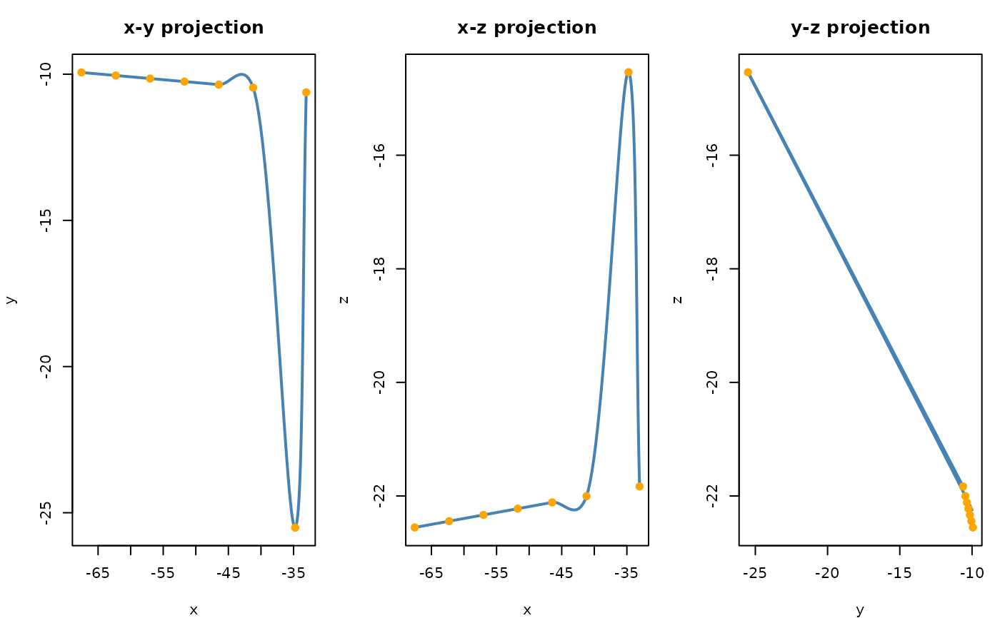
plot(curve, use_rgl = FALSE)