Common Average Re-referencing by Least Anti-Correlation (CARLA)

Selects an optimal subset of channels to use as the common average reference (CAR) for cortico-cortical evoked potential (CCEP) data, following the CARLA (see 'Reference' and 'Citation'). Channels are ranked in increasing order of their cross-trial covariance (or variance when only one trial is available); subsets are then iteratively grown and the size that yields the least anti-correlation between the candidate reference and the remaining unreferenced channels is selected as optimal.

Usage

carla(
  x,
  nboot = 100L,
  sensitive = FALSE,
  min_size = NULL,
  absolute_rank = FALSE,
  virtual_reference = FALSE
)

Arguments

x: numeric array of shape channels x time x trials; if a matrix is provided, it is treated as channels x time (single trial). The signal must already be cropped to the responsive time window (typically 0.01 s to 0.3 s post-stimulus).
nboot: integer, number of bootstrapped trial resamplings used to estimate the optimization statistic; defaults to 100. Ignored when a single trial is supplied.
sensitive: logical; if TRUE (and more than one trial is supplied), the more sensitive cutoff is used, corresponding to the channel count just before the first statistically significant decrease in the mean anti-correlation curve. The default FALSE returns the global maximum of that curve.
min_size: integer, minimum subset size considered when sensitive = TRUE; defaults to max(2, ceiling(0.1 * nchan_good)), where nchan_good is the number of usable channels after the bad-channel mask has been applied (see Details). Floored at 2 because subset size 1 is never evaluated.
absolute_rank: logical; if FALSE (the default), the per-channel ranking statistic is the signed mean of the off-diagonal trial-to-trial covariances, as in the original CARLA manuscript. This assumes a phase-locked evoked response, so trial-pair covariances on responsive channels are positive and a clean signed mean separates them from non-responsive channels. Set to TRUE to use the mean of the absolute covariances instead, which is more robust to evoked responses whose polarity flips across trials (e.g. alternating-polarity stimulation, biphasic CCEPs with jitter), at the cost of an upward bias on the non-responsive floor. Ignored when only one trial is supplied (the per-channel variance is used in that case).
virtual_reference: logical; if TRUE, runs the modified CARLA before the iterative subset evaluation: rank channels once, designate the channel with the median rank as a "virtual reference", subtract its signal from every channel, then re-rank on the subtracted data. The virtual channel itself is pinned to the very end of the new ordering so it is never picked into the CAR until the final subset size. This is intended for data where the recording reference is contaminated by stimulation artifact or evoked activity: a contaminated reference makes every channel look artificially similar and biases the covariance/variance ranking statistic, but subtracting a mid-rank proxy of that contamination unbiases the ranking so genuinely responsive channels rise to the top. Default FALSE reproduces the original CARLA algorithm bit-for-bit.

Value

A list with the following elements:

channels: integer vector, sorted indices (1-based) of the channels chosen to construct the common average reference.
car: numeric matrix of shape time x trials (or numeric vector when only one trial is supplied) holding the common average signal computed from channels. Subtract this from each channel of the original signal to obtain the re-referenced data.
order: integer vector, indices of the good channels sorted in increasing order of the ranking statistic. Bad channels (zero variance / all-NA; see Details) are excluded.
vars: numeric vector of length nchan containing the per-channel ranking statistic (mean cross-trial covariance, or variance for a single trial). Bad channels keep their raw value (zero or NA) so callers can audit the mask.
n_optimum: integer, the optimal subset size selected (indexes into order).
zmin_mean: numeric matrix of shape length(order) x nboot (or a length-length(order) vector for a single trial / nboot = 1) holding, for each subset size and bootstrap, the mean Fisher z-transformed correlation of the most globally anti-correlated unreferenced channel against the candidate CAR. Row 1 is always NA (subset size 1 is not evaluated).
bad_channels: integer vector of channel indices that were excluded from the analysis because their ranking statistic was zero or NA (flat / dead channels, plus the virtual channel itself when virtual_reference = TRUE).
virtual_channel: integer, the index (1-based) of the channel used as the virtual reference when virtual_reference = TRUE; NA_integer_ otherwise.
vars1: numeric vector of the first-pass ranking statistic when virtual_reference = TRUE (the post-subtraction statistic is returned in vars); NULL otherwise.

Details

The function is a faithful port of the core CARLA.m routine; it does not perform notch filtering, time-window cropping, or grouping by stimulation site. Those steps belong to the surrounding preprocess pipeline (see the example below).

For each candidate subset size \(n = 2, \ldots, N\), the candidate reference is computed as the channel-wise mean of the \(n\) lowest-ranked channels. Each of those \(n\) channels is then correlated, in its unreferenced form, against every channel of the candidate re-referenced subset. The resulting Pearson correlations are Fisher z-transformed; the row corresponding to the most globally anti-correlated channel is recorded as zmin. The optimal \(n\) is the one that maximizes (i.e. makes least negative) the mean of zmin.

Bad-channel mask. Channels whose ranking statistic is exactly zero or NA are flagged as "bad" and excluded both from the CAR candidate pool and from the target-channel correlation rows. This catches flat / dead channels (constant signal, no usable variance) and , when virtual_reference = TRUE, automatically removes the virtual channel itself, since subtracting it from itself yields a zero trace. All references to channel indices in the returned order, n_optimum, and zmin_mean are with respect to the good channels only; vars is full-length so callers can inspect the raw scores.

References

The CARLA algorithm (virtual_reference = FALSE) is described in doi:10.1016/j.jneumeth.2024.110153 ; the modified CARLA precursor (virtual_reference = TRUE) is described in doi:10.1016/j.jneumeth.2025.110461 , with a reference implementation at https://github.com/hharveygit/SPES_reference_contam. See citation("ravetools") for the full bibliographic entries of both manuscripts.

Examples


# ---- Simulate a small CCEP-like dataset --------------------------------
# 16 channels, 12 trials, sampled at 1 kHz, 0.5 s peri-stimulus epoch.
# Channels 1:4 are "responsive" (carry an evoked potential); the rest are
# noise-only and should make up the optimal CAR.
srate <- 1000
tt <- seq(-0.1, 0.4 - 1 / srate, by = 1 / srate)   # time, seconds
nchan <- 16
ntrial <- 30
resp_ch <- 1:4
noise_ch <- 4:7

# Evoked potential template: damped sinusoid starting at t = 0
ep <- ifelse(tt >= 0,
             80 * exp(-tt / 0.05) * sin(2 * pi * 12 * tt),
             0)

# channels x time x trials
x_full <- array(rnorm(nchan * length(tt) * ntrial, sd = 5),
                dim = c(nchan, length(tt), ntrial))
for (ch in resp_ch) {
  for (k in seq_len(ntrial)) {
    x_full[ch, , k] <- x_full[ch, , k] + ep * runif(1, -0.8, 1.2)
  }
}
for (ch in noise_ch) {
  for (k in seq_len(ntrial)) {
    tmp <- x_full[ch, , k]
    x_full[ch, , k] <- tmp + sign(ch %% 2 - 0.5) * 5 *
      runif(length(tmp), 0.8, 1.2)
  }
}
# Add artifacts common to all channels and trials
artifacts <- 6 * sin(2 * pi * 60 * tt) + 7 * sin(2 * pi * 24 * tt)
x_full <- sweep(x_full, 2L, artifacts, "+")

# ---- 1. Notch filter line noise (per channel, per trial) ---------------
# The CARLA paper notch-filters before ranking; the re-reference itself
# is applied to the original (unfiltered) signal.
x_clean <- x_full
for (ch in seq_len(nchan)) {
  for (k in seq_len(ntrial)) {
    x_clean[ch, , k] <- notch_filter(
      x_full[ch, , k], sample_rate = srate,
      lb = c(59, 119, 179), ub = c(61, 121, 181)
    )
  }
}

# ---- 2. Crop to the responsive window (0.01 s to 0.3 s post-stim) ------
resp_idx <- which(tt > 0.0 & tt <= 0.3)
x_resp <- x_clean[, resp_idx, , drop = FALSE]

# ---- 3. Run CARLA to pick reference channels ---------------------------
fit <- carla(x_resp, sensitive = TRUE, absolute_rank = TRUE,
             virtual_reference = TRUE)
fit$channels        # selected reference channels (should exclude 1:4)
#>  [1]  5  6  7  8  9 10 11 13 14 15 16
fit$n_optimum       # number of channels in the optimal CAR
#> [1] 11

# ---- 4. Re-reference the ORIGINAL (unfiltered) signal ------------------
# mean or median, your choice!
car_full <- apply(x_full[fit$channels, , , drop = FALSE], c(2, 3), mean)

# old-style: using all channels for CAR
car_old <- apply(x_full, c(2, 3), mean)

x_reref <- sweep(x_full, c(2, 3), car_full, "-")
x_compare <- sweep(x_full, c(2, 3), car_old, "-")

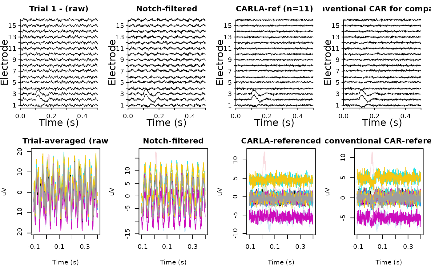
# ---- 5. Inspect: evoked potential is preserved on responsive channels --
op <- graphics::par(mfrow = c(2, 4), mar = c(4, 4, 2, 1))
ravetools::plot_signals(
  signals = x_full[, , 1],
  sample_rate = srate,
  main = "Trial 1 - (raw)")

ravetools::plot_signals(
  signals = x_clean[, , 1],
  sample_rate = srate,
  main = "Notch-filtered")

ravetools::plot_signals(
  signals = x_reref[, , 1],
  sample_rate = srate,
  main = sprintf("CARLA-ref (n=%d)", length(fit$channels)))

ravetools::plot_signals(
  signals = x_compare[, , 1],
  sample_rate = srate,
  main = "Conventional CAR for comparison")

col <- adjustcolor(seq_len(nchan))
col[resp_ch] <- adjustcolor(col[resp_ch], alpha.f = 0.2)

graphics::matplot(tt, t(rowMeans(x_full, dims = 2L)),
                  type = "l", lty = 1, xlab = "Time (s)", ylab = "uV",
                  main = "Trial-averaged (raw", col = col)

graphics::matplot(tt, t(rowMeans(x_clean, dims = 2L)),
                  type = "l", lty = 1, xlab = "Time (s)", ylab = "uV",
                  main = "Notch-filtered", col = col)

graphics::matplot(tt, t(rowMeans(x_reref, dims = 2L)),
                  type = "l", lty = 1, xlab = "Time (s)", ylab = "uV",
                  main = "CARLA-referenced", col = col)

graphics::matplot(tt, t(rowMeans(x_compare, dims = 2L)),
                  type = "l", lty = 1, xlab = "Time (s)", ylab = "uV",
                  main = "conventional CAR-referenced", col = col)


graphics::par(op)