Stores large arrays in files to avoid occupying large memories. Implemented with super fast gigabyte-level multi-threaded reading/writing via OpenMP. Supports multiple non-character data types (double, float, integer, complex, logical and raw).

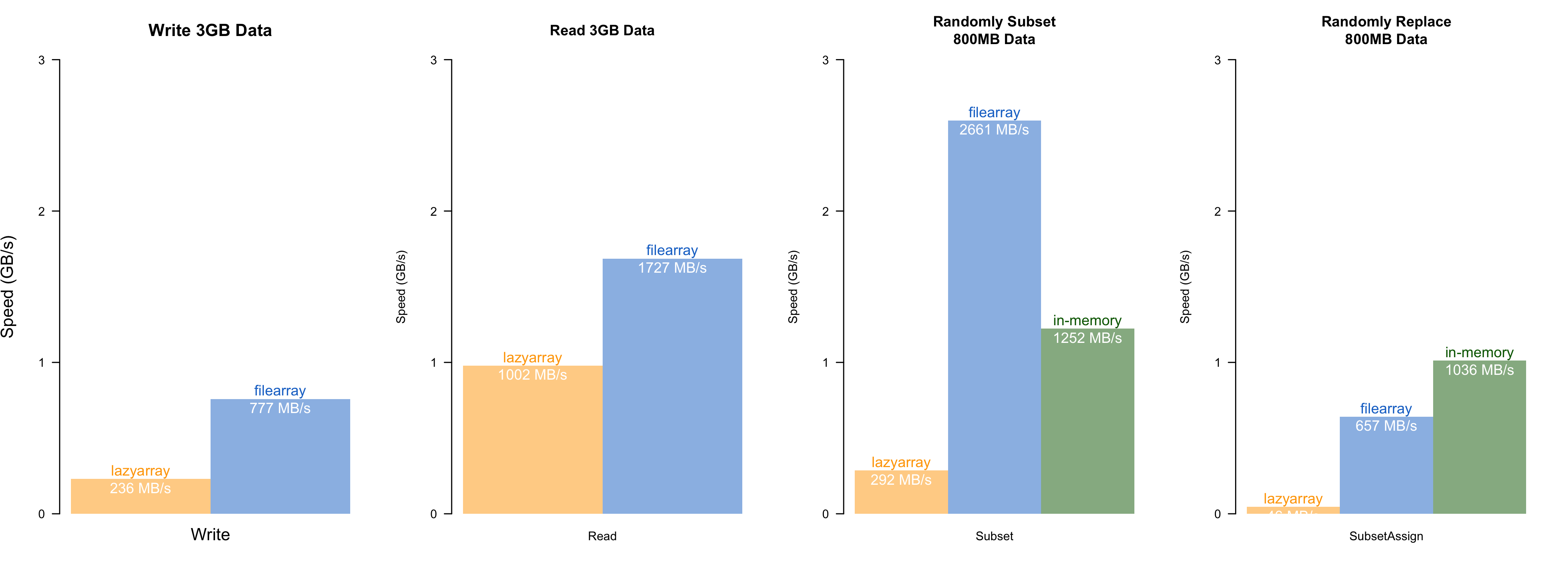
Speed comparisons with lazyarray (zstd-compressed out-of-memory array), and in-memory operation. The speed test was conducted on an MacBook Air (M1, 2020, 8GB RAM), with 8-threads. filearray is uniformly faster than lazyarray. Random access has almost the same speed as the native array operation in R. (The actual speed may vary depending on the storage type and memory size)
Installation
install.packages("filearray")Install Develop Version
The internal functions are written in C++. To avoid compiling the packages, you can install from my personal repository. It’s automatically updated every hour. Currently available on Windows and osx (Intel chip) only.
options(repos = c(
    dipterix = 'https://dipterix.r-universe.dev',
    CRAN = 'https://cloud.r-project.org'))

install.packages('filearray')
Alternatively, you can compile from Github repository. This requires proper compilers (rtools on windows, or xcode-select --install on osx, or build-essentials on linux).
# install.packages("remotes")
remotes::install_github("dipterix/filearray")
Basic Usage
Create/load file array
library(filearray)
file <- tempfile()
x <- filearray_create(file, c(100, 100, 100, 100))

# load existing
x <- filearray_load(file)
See more: help("filearray")
Assign & subset array
x[,,,1] <- rnorm(1e6)
x[1:10,1,1,1]
Generics
typeof(x)
max(x, na.rm = TRUE)
apply(x, 3, min, na.rm = TRUE)

val = x[1,1,5,1]
fwhich(x, val, arr.ind = TRUE)
See more: help("S3-filearray"), help("fwhich")
Map-reduce
Process segments of array and reduce to save memories.
# Identical to sum(x, na.rm = TRUE)
mapreduce(x,
          map = \(data){ sum(data, na.rm = TRUE) },
          reduce = \(mapped){ do.call(sum, mapped) })
See more: help("mapreduce")
Collapse
Transform data, and collapse (calculate sum or mean) along margins.
a <- x$collapse(keep = 4, method = "mean", transform = "asis")

# equivalent to
b <- apply(x[], 4, mean)

a[1] - b[1]
Available transform for double/integer numbers are:
-
asis: no transform -
10log10:10 * log10(v) -
square:v * v -
sqrt:sqrt(v)
For complex numbers, transform is a little bit different:
-
asis: no transform -
10log10:10 * log10(|x|^2)(power to decibel unit) -
square:|x|^2 -
sqrt:|x|(modulus) -
normalize:x / |x|(unit length)
Notes
I. Notes on precision
complexnumbers: In nativeR, complex numbers are combination of twodoublenumbers - real and imaginary (total 16 bytes). Infilearray, complex numbers are coerced to twofloatnumbers and store each number in 8 bytes. This conversion will gain performance speed, but lose precision at around 8 decimal place. For example,1.0000001will be store as1, or123456789will be stored as123456792(first 7 digits are accurate).floattype: Native R does not have float type. All numeric values are stored in double precision. Since float numbers use half of the space, float arrays can be faster when hard drive speed is the bottle-neck (see performance comparisons). However coercing double to float comes at costs: a). float number has less precision b). float number has smaller range () than double () hence use with caution when data needs high precision or the max is super large.collapsefunction: when data range is large (sayx[[1]]=1, butx[[2]]=10^20),collapsemethod might lose precision. This isdoubleonly uses 8 bytes of memory space. When calculating summations, R internally useslong doubleto prevent precision loss, but currentfilearrayimplementation usesdouble, causing floating error around 16 decimal place.
II. Cold-start vs warm-start
As of version 0.1.1, most file read/write operations are switched from fopen to memory map for two simplify the logic (buffer size, kernel cache…), and to boost the writing/some types of reading speed. While sacrificing the speed of reading large block of data from 2.4GB/s to 1.7GB/s, the writing speed was boosted from 300MB/s to 700MB/s, and the speed of random accessing small slices of data was increased from 900MB/s to 2.5GB/s. As a result, some functions can reach to really high speed (close to in-memory calls) while using much less memory.
The additional performance improvements brought by the memory mapping approach might be impacted by “cold” start. When reading/writing files, most modern systems will cache the files so that it can load up these files faster next time. I personally call it a cold start. Memory mapping have a little bit extra overhead during the cold start, resulting in decreased performance (but it’s still fast). Accessing the same data after the cold start is called warm start. When operating with warm starts, filearray is as fast as native R arrays (sometimes even faster due to the indexing method and fewer garbage collections). This means filearray reaches its best performance when the arrays are re-used.
III. Using traditional HDD?
filearray relies on SSD, especially NVMe SSD that allows you to fast-access random hard disk address. If you use HDD, filearray can provide very limited improvement.
If you use filearray to direct access to HDD, please set number of threads to 1 via filearray::filearray_threads(1) at start up, or set system environment FILEARRAY_NUM_THREADS to "1".