1. %?<-%: Assign if invalid
When coding in R, the data checking is actually a headache. For
example, to check if a variable aa exists and not
NULL, otherwise set a default value to be 1, the check
looks like:
Most of time we are repeating ourselves. With %?<-%
operator, we just need:
The powerful part is the left-hand side can be any expression. For example,
If the value exists, then %?<-% does nothing (not
even evaluate the expressions on the right-hand side)
2. JavaScript-style of creating functions
In modern JavaScript, function can be created via
(arg) => { ... }. For example,
dipsaus provides functions iapply, and
%=>%, for example:
li <- c('A', 'T', 'G', 'C')
li |> iapply(alist(el, ii) %=>% {
  sprintf('The index for %s is %s', el, ii)
})
#> [1] "The index for A is 1" "The index for T is 2" "The index for G is 3"
#> [4] "The index for C is 4"
%=>% collect the left-hand side elements as arguments
and right-hand side expression as body and create function:
3. Match nested calls match_calls
The function match.call provided by base package let us
format calls with formals matched.
match.call(textInput, call = quote(textInput('inputId', 'label', 'aaa')))
#> textInput(inputId = "inputId", label = "label", value = "aaa")
This is already powerful as we can parse the expressions using
as.list() to get the input parameters. However, when
encounter the nested calls like shiny UI components,
match.call does not work well. We can’t see the matched
results inside of the nested functions.
match.call(tagList, call = quote(tagList(
  div(
    tags$ul(
      tags$li(textInput('inputId', 'label', 'aaa'))
    )
  )
)))
#> tagList(div(tags$ul(tags$li(textInput("inputId", "label", "aaa")))))
match_calls solves this problem by recursively calling
match.call:
match_calls(call = tagList(
  div(
    tags$ul(
      tags$li(textInput('inputId', 'label', 'aaa'))
    )
  )
), recursive = TRUE)
#> tagList(div(tags$ul(tags$li(textInput(inputId = "inputId", label = "label",
#>     value = "aaa")))))
It can also change modify the calls. For example, we want to add
ns to input ID in shiny modules, then the following
replave_args changes "inputId" to
ns("inputId")
match_calls(call = tagList(
  div(
    tags$ul(
      tags$li(textInput('inputId', 'label', 'aaa'))
    )
  )
), recursive = TRUE, replace_args = list(
  'inputId' = function(v, ...){
    as.call(list(quote(ns), v))
  }
))
#> tagList(div(tags$ul(tags$li(textInput(inputId = ns("inputId"),
#>     label = "label", value = "aaa")))))
4. Pipe-friendly functions
Pipe functions can simplify the workflow and make R code more
readable. The popular pipe operator %>% (or
|> after R 4.0) allows the left-hand elements to be the
first input of the right-hand side functions. dipsaus
provides several pipe-friendly functions.
No-operations no_op
no_op takes whatever input in, and returns the input,
with side effects. For example, we want to plot the results from the
pipe and continue the analysis, usually this is what happens:
x_tmp <- x |>
  do_something(...)

plot(x_tmp)

final_results <- x_tmp |>
  do_others(...)
With no_op, the pipe becomes:
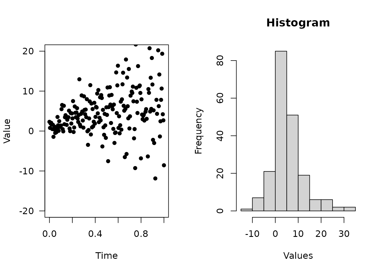
Here’s an example
par(mfrow = c(1,2))

result <- (1:10) |>
  iapply(alist(el, ii) %=>% {
    rnorm(20, el, ii)
  }, simplify = FALSE) |>
  unlist() |>

  # Begin no-ops, result will not change
  no_op({
    # Use expression and "." to refer the data
    print(summary(.))
  }) |>
  no_op(
    # Use function and pass ... to function
    plot, x = seq(0,1,length.out = 200),
    type = 'p', ylim = c(-20,20), pch = 16,
    xlab = 'Time', ylab = 'Value', las = 1
  ) |>
  no_op(hist, xlab = 'Values', main = 'Histogram')
#>    Min. 1st Qu.  Median    Mean 3rd Qu.    Max.
#>  -8.101   1.379   4.588   6.344  10.196  35.644
str(result)
#>  num [1:200] -0.4 1.255 -1.437 0.994 1.622 ...
do_aggregate
This is a wrapper of aggregate function. When using
formula, aggregate requires the formula to be the first
element. If the pipe results are data.frame and we want to
use formula, it’s super inconvenient.
## S3 method for class 'formula'
aggregate(formula, data, FUN, ..., subset, na.action = na.omit)
do_aggregate allows the first element to be data frames
while using formula:
ToothGrowth |>
  do_aggregate(len ~ ., mean)
#>   supp dose   len
#> 1   OJ  0.5 13.23
#> 2   VC  0.5  7.98
#> 3   OJ  1.0 22.70
#> 4   VC  1.0 16.77
#> 5   OJ  2.0 26.06
#> 6   VC  2.0 26.14