Plot '3D' surface objects

Usage

# S3 method for class 'ieegio_surface'
plot(
  x,
  method = c("basic", "full"),
  transform = 1L,
  name = "auto",
  vlim = NULL,
  col = c("black", "white"),
  slice_index = NULL,
  ...
)

Arguments

x: 'ieegio_surface' object, see read_surface
method: plot method; 'basic' for just rendering the surfaces; 'full' for rendering with axes and title
transform: which transform to use, can be a 4-by-4 matrix; if the surface contains transform matrix, then this argument can be an integer index of the transform embedded, or the target (transformed) space name; print names(x$transforms) for choices
name: attribute and name used for colors, options can be 'color' if the surface has color matrix; c('annotations', varname) for rendering colors from annotations with variable varname; c('measurements', varname) for rendering colors from measurements with variable varname; 'time_series' for plotting time series slices; or "flat" for flat color; default is 'auto', which will plot the first available data. More details see 'Examples'.
vlim: when plotting with continuous data (name is measurements or time-series), the value limit used to generate color palette; default is NULL: the range of the values. This argument can be length of 1 ( creating symmetric value range) or 2. If set, then values exceeding the range will be trimmed to the limit
col: color or colors to form the color palette when value data is continuous; when name="flat", the last color will be used
slice_index: when plotting the name="time_series" data, the slice indices to plot; default is to select a maximum of 4 slices
...: ignored

Examples





library(ieegio)

# geometry
geom_file <- "gifti/GzipBase64/sujet01_Lwhite.surf.gii"

# measurements
shape_file <- "gifti/GzipBase64/sujet01_Lwhite.shape.gii"

# time series
ts_file <- "gifti/GzipBase64/fmri_sujet01_Lwhite_projection.time.gii"

if(ieegio_sample_data(geom_file, test = TRUE)) {

  geometry <- read_surface(ieegio_sample_data(geom_file))
  measurement <- read_surface(ieegio_sample_data(shape_file))
  time_series <- read_surface(ieegio_sample_data(ts_file))
  ts_demean <- apply(
    time_series$time_series$value,
    MARGIN = 1L,
    FUN = function(x) {
      x - mean(x)
    }
  )
  time_series$time_series$value <- t(ts_demean)

  # merge measurement & time_series into geometry (optional)
  merged <- merge(geometry, measurement, time_series)
  print(merged)

  # ---- plot method/style ------------------------------------
  plot(merged, "basic")
  plot(merged, "full")

  # ---- plot data --------------------------------------------

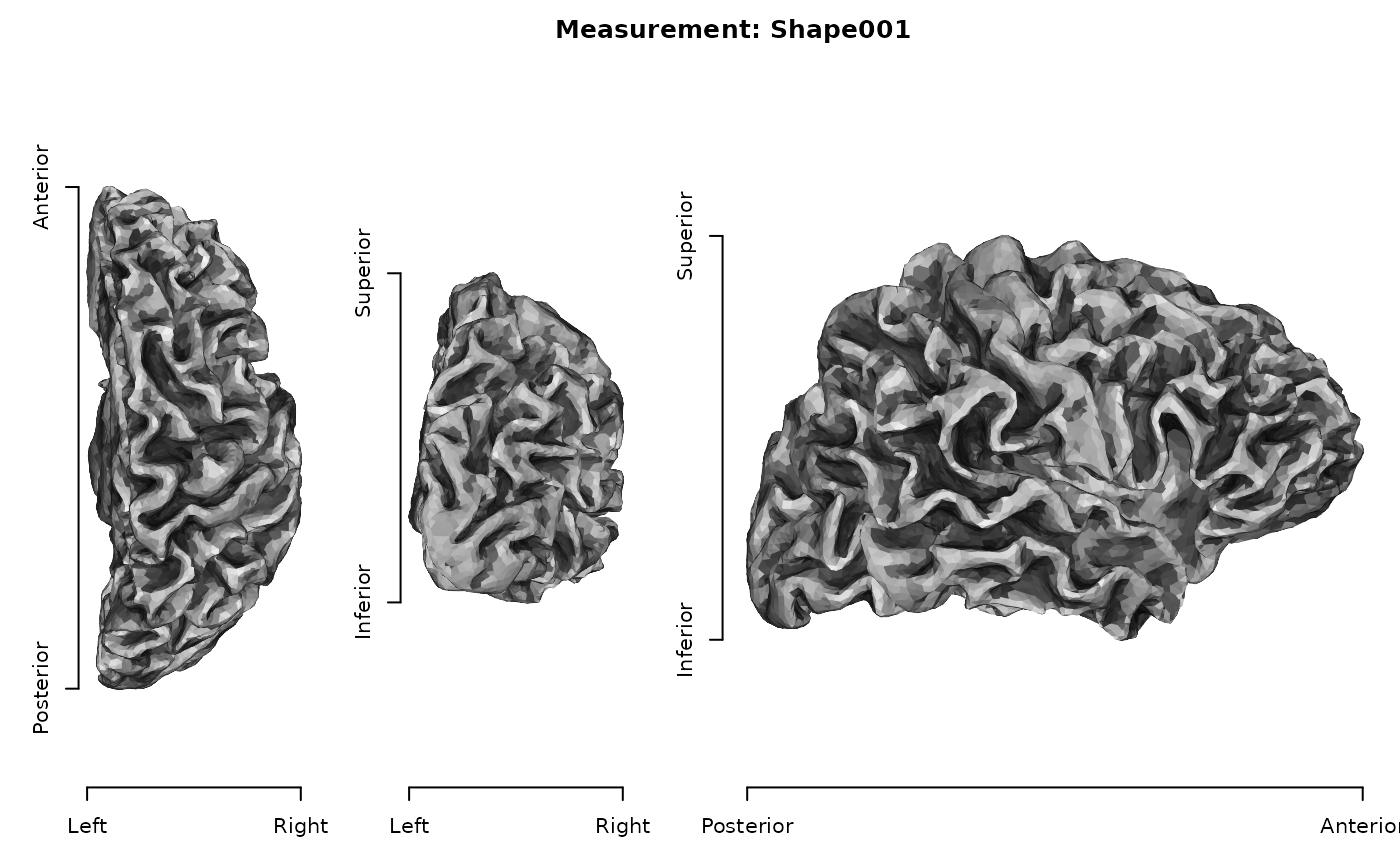
  ## Measurements or annotations

  # the first column of `measurements`
  plot(merged, name = "measurements")

  # equivalent to
  plot(merged, name = list("measurements", 1L))

  # equivalent to
  measurement_names <- names(merged$measurements$data_table)
  plot(merged, name = list("measurements", measurement_names[[1]]))

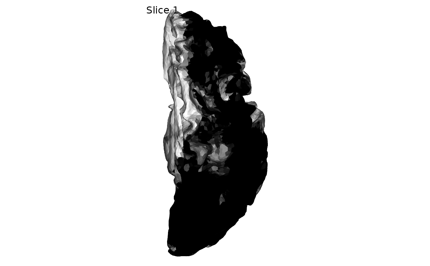
  ## Time-series

  # automatically select 4 slices, trim the color palette
  # from -25 to 25
  plot(merged, name = "time_series", vlim = c(-25, 25))

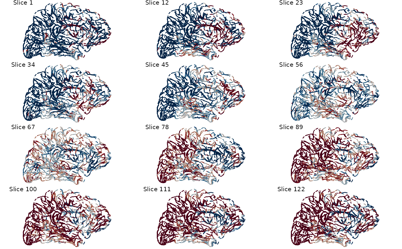
  plot(
    merged,
    name = "time_series",
    vlim = c(-25, 25),
    slice_index = c(1, 17, 33, 49, 64, 80, 96, 112, 128),
    col = c("#053061", "#2166ac", "#4393c3",
            "#92c5de", "#d1e5f0", "#ffffff",
            "#fddbc7", "#f4a582", "#d6604d",
            "#b2182b", "#67001f")
  )


}